Module 8 Example: Creating a project template

For this module, we’ll show an example of creating a project directory template for a lab group. We will walk through the process of creating a project directory template that could be used to manage and analyze data from any of the specific studies for this group. We’ll start by discussing the steps of the conceptual design—figuring out how a blueprint for the standard subdirectories and the file naming conventions. We’ll then show how this blueprint can be developed into physical implementation: a file directory that can be copied and renamed to initiate a new project. The full directory of files for this example can be found at https://github.com/geanders/example_for_improve_repro, where you can download them or explore them online.

Objectives. After this module, the trainee will be able to:

• Examine files from previous projects as a step in developing a project directory template
• Develop a structure of subdirectories for a project directory template
• Create a project directory template to initialize consistently-formatted directories for a lab group’s experiments
• Explain how a report template can be incorporated within a project directory template

8.1 Description of the example set of studies

In this module, we’ll use an example based on a set of real immunology experiments. This example highlights how a research laboratory will often conduct a similar type of experiment many times, so it lets us demonstrate how a project directory template can be reused across similar experiments. It will allow us to show you how you can move from designing a file directory for a single experiment to designing one that can be used repeatedly, and then how you can take advantage of consistency in the directory structure across projects to make templates for data collection that can be reused.

This example covers a group of studies that explored novel treatments for tuberculosis. While treatments exist for tuberculosis, the current treatment regime is lengthy and involves a combination of multiple drugs. If the treatment is not completed, it can result in the development and spread of drug-resistant tuberculosis strains, and so the treatment sometimes must be done under observation.¹⁸⁷ If the patient has a strain of tuberculosis that is resistant to first-line drugs, they need to be treated with second-line drugs, which can have serious side effects.¹⁸⁸ There is a critical need to develop more candidate drugs against this disease, given all the limitations and struggles of the current treatment regime.

Each study investigates how mice challenged with tuberculosis respond to different treatments, both in terms of how well they handle the treatment (assessed by checking if their weight decreases notably while on treatment) and also how well the treatment manages to limit the growth of tuberculosis in the mouse’s lungs.

These example studies were conducted with similar designs and similar goals—all aimed to test candidate treatments for tuberculosis. Most studies in this set tested one or more treatments as well as one or more controls. The controls could include negative controls, like saline solution, or positive controls, like a drug already in use to treat the disease (e.g., isoniazid). A few of the studies tested only controls, to develop baseline expectations for things like the bacterial load in different mouse strains. The set of studies tested some treatments that were monotherapies (only one drug given to the animal) as well as some that were combinations of two or three drugs. For many of the drugs that were tested, they were tested at different doses and, in some cases, different methods of delivery or different mouse models.

Each of the treatments were given to several mice that had been infected with Mycobacterium tuberculosis. During the treatment, the mice were weighed regularly. This weight measurement helps to determine if a particular treatment is well-tolerated by the animals—if not, it may show through the treated mice losing weight during treatment. For convenience, the mice were not weighed individually. Instead, mice with the same treatment were kept in a single cage, and the entire cage was weighed, the weight of the cage itself factored out, and the average weight of mice determined by dividing by the number of mice in the cage. After a period of time, the mice were sacrificed and one lobe from their lungs was used to determine each mouse’s bacterial load, through plating the material from the lobe and counting the colony forming units (CFUs). One aim of the data analysis is to compare the bacterial load of mice under various treatments to the bacterial load of mice in the control group.

The full set of studies included 19 studies. These were conducted at different times, but the data for all of the studies can be collected using a common format, and we’ll talk about how both data collection templates and a project directory template could be designed to accomodate these experiments.

8.2 Step 1: Survey of data collected for the projects

The first step in developing a project template is to survey the typical types of files that are included in your research projects. To give an example of this part of the design process, let’s walk through the types of data that were collected for the example studies.

First, there were metadata recorded for each study. Figure 8.1 gives an example. This includes information about the strain of mouse that was used in the study, treatment details (including the method of giving the drug or drugs, how often they were given each week, and for how many weeks), how much bacteria the animals were exposed to (measured both in terms of the inoculum they were given and their bacterial load one day after they were given that inoculum, which was based on sacrificing one animal the day after challenging all the animals with the bacteria), and, if the study included a novel drug as part of the tested treatment, the batch number of that drug.

Figure 8.1: Example of recording metadata for a study in the set of example studies for this module.

Next, the researchers recorded some information about each treatment group within the experiment. This typically included at least one negative control. In some cases, there was also a positive control, in which the animals were treated with a drug that’s in standard use against tuberculosis already (e.g., isoniazid). Most studies would also test one or more treatments, which could include monotherapies or combined therapies. Figure 8.2 shows an example of the data that were recorded on each treatment in the study. These data include the names and doses of up to three drugs in each treatment, as well as a column where the researcher can provide detailed specifications of the treatment.

Figure 8.2: Example of recording treatment details for a study in the set of example studies for this module.

Once the animals were challenged with the bacteria, treatment began, and two main types of data were measured and recorded. First, the mice were weighed once a week. For convenience, the mice were not weighed individually. Instead, mice with the same treatment were kept in a single cage, and the entire cage was weighed, the weight of the cage itself factored out, and the average weight of mice for that treatment determined by dividing the weight of all mice in the cage by the number of mice in the cage. These weights were converted to a measure of the percent change in weight since the start of treatment. If the animals’ weights decrease during the treatment, it is a marker that the treatment is not well-tolerated by the animals. Figure 8.3 shows an example of how these data could be recorded. All animals within a treatment group were kept in the same cage, and this cage was measured once a week. By dividing the weight of all animals in the cage by the number of animals, the researchers could estimate the average weight of animals in that treatment group, which is recorded as shown in Figure 8.3.

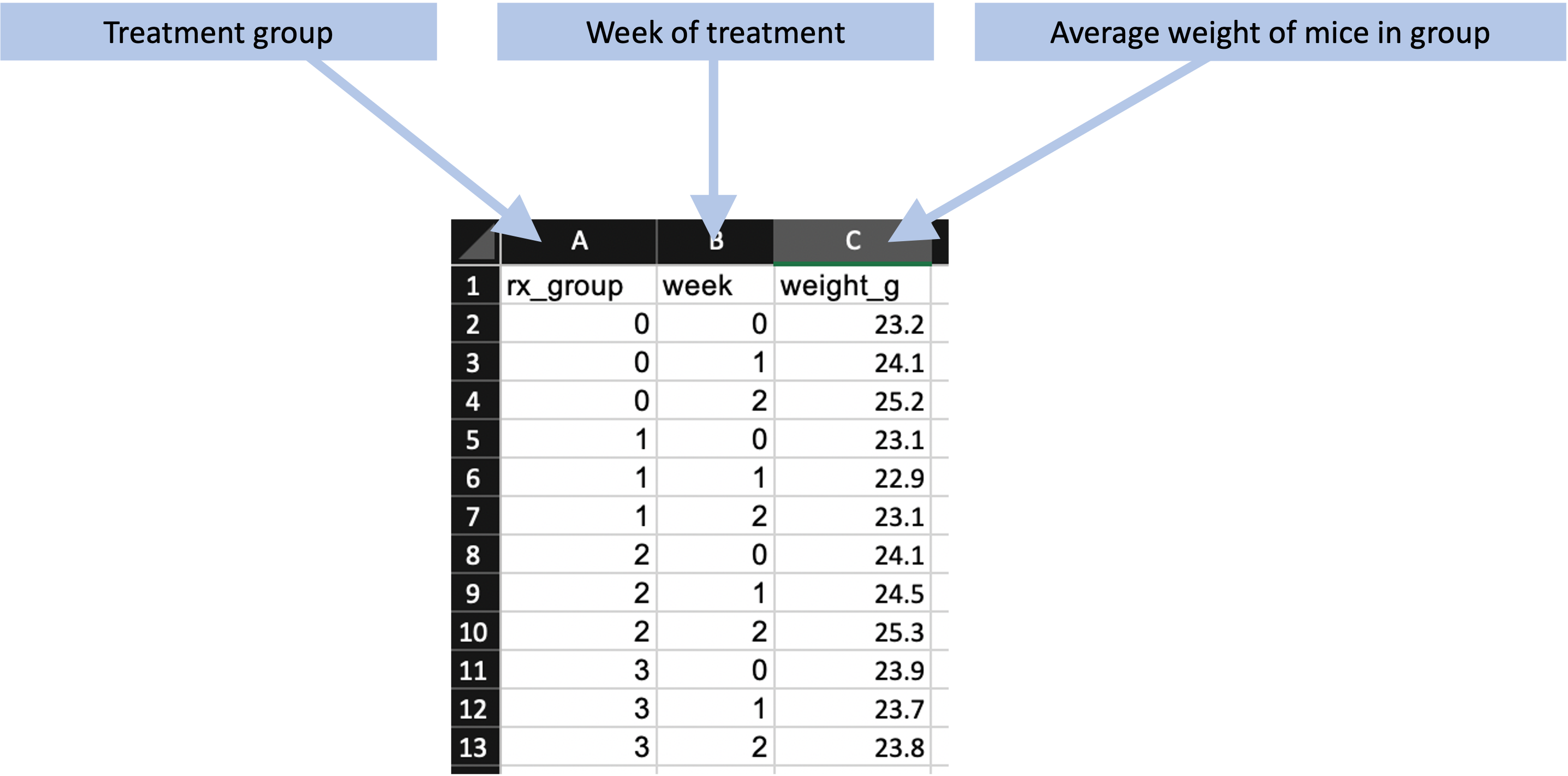
Figure 8.3: Example of recording weekly weights of mice in each treatment group for the example set of studies.

Finally, after the treatment period, the mice were sacrificed and a portion of each mouse’s lung was used to estimate the bacterial load in that mouse. Figure 8.4 shows an example of how the data on the bacterial load in each mouse can be recorded.

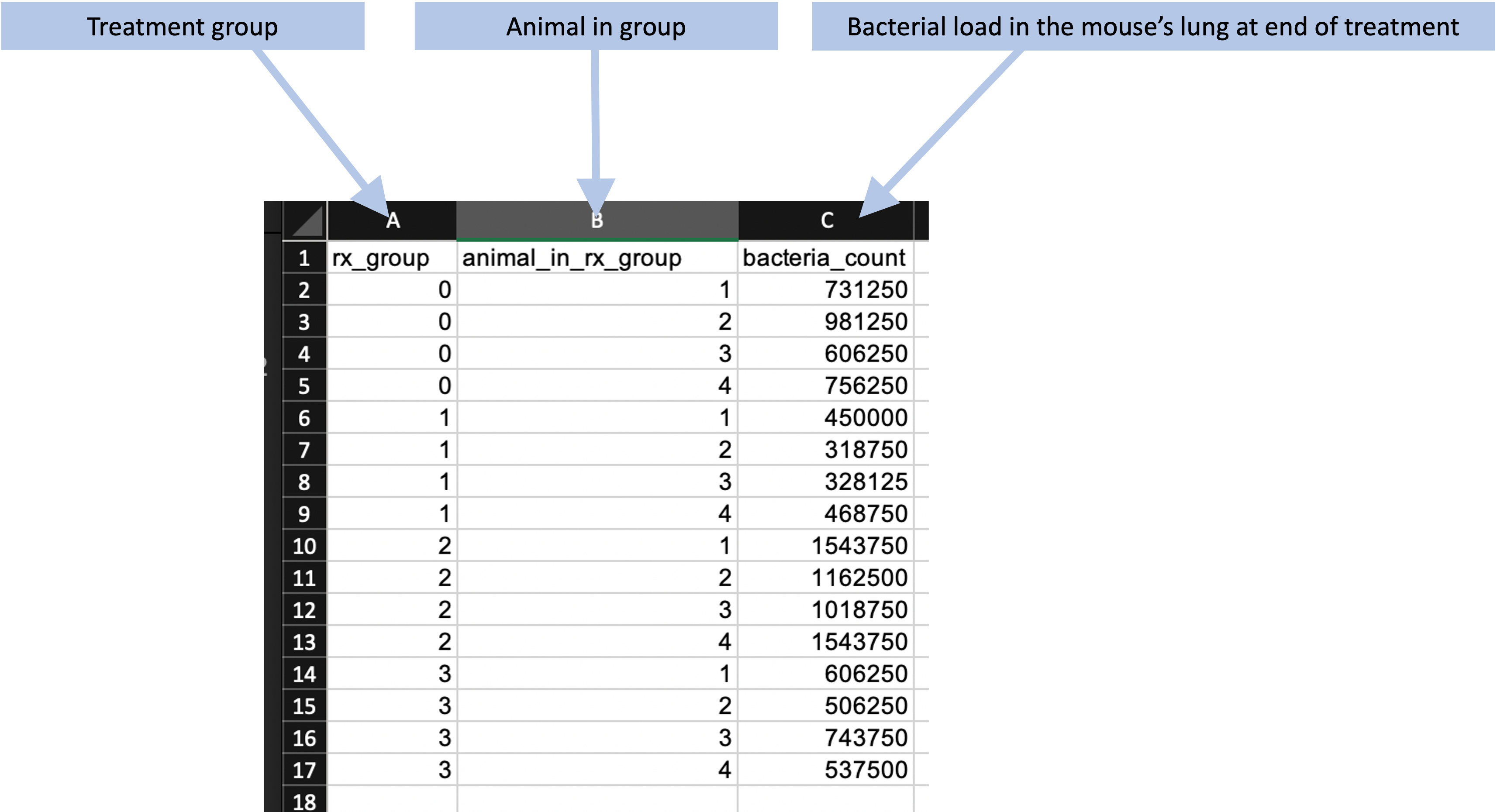
Figure 8.4: Example of recording the bacterial load in the lungs of each mouse at the end of treatment for the example set of studies.

These examples are all data that the researchers record by entering them on spreadsheets. It is helpful at this stage to ensure this type of data is recorded in a way that separates data recording and analysis (module 2). The example files we’ve shown here do—there are no extra elements in these spreadsheets that do calculations or create graphs. Later in this module, we’ll talk a bit more about how these templates can be designed as part of the process of designing the full project directory template. Earlier modules (modules 4 and 5) provide more focused details on designing data collection templates like these.

Another type of files that the group’s studies typically generate are ones that are generated directly by laboratory equipment. For example, their experiments may include flow cytometry assays, with files output in a specialized format directly from the flow cytometer. Some experiments might also collect data through single-cell RNA sequencing. We’ll want to keep these files in mind as we design the structure of the project directory template.

8.3 Step 2: Organizing a project directory

Once you’ve determined the types of files that you’ll normally include in your project, you then need to decide how to organize them into subdirectories in the project file directory. In this case, we’ve organized the project directory template to include just a few things at the top level (Figure 8.5, also shown in module 7):

• A spreadsheet that stores meta-data about the experiment
• A subdirectory named “raw_data”, where we’ll store original raw files of data, before it is pre-processed, focusing on data generated by laboratory equipment
• A subdirectory named “data”, which will store experimental data once it has been pre-processed, as well as recorded data that do not require pre-processing
• A subdirectory named “R”, which will store code for pre-processing and analysis
• A subdirectory named “reports”, which will store the files to generate reports, as well as any reports that are ultimately generated

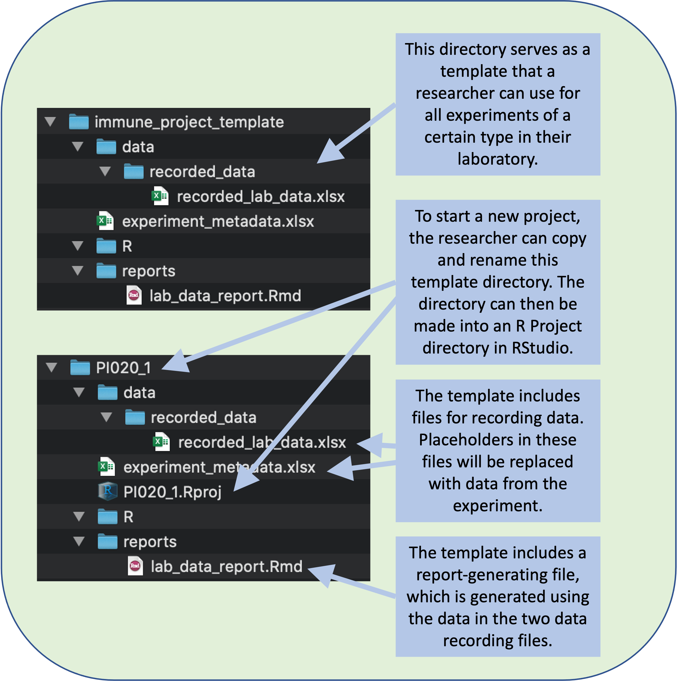
Figure 8.5: A research group can create a file directory that will serve as a template for all the experiments of a certain type in your laboratory. The template can include templates of files for data recording and for generating reports. To start recording data for a new experiment, a researcher can copy and rename this template directory.

You may have noticed that this structure captures each of the main elements that we discussed including in a project template in module 7: data, code, reports, and metadata.

In this structure, we’ve selected subdirectory names that are generic enough (e.g., “data”, “reports”) that they can be reused across many of our projects without modification. These names should also be clear to any researcher that explores this directory in the future, since the names are clear and unambiguous. However, you might make different choices—for example, if some of your team aren’t familiar with R as a programming language, you may want to use the subdirectory name “code” rather than “R”.

Within some of the subdirectories, we can include more subdirectories to further organize files (Figure8.6, repeated from module 7). For example, within the “data” subdirectory, we can have subdirectories for different types of data:

• A subdirectory named “flow_data” for data from flow cytometry
• A subdirectory named “recorded_data”, for data that are recorded “by hand” in the laboratory (for example, the weights of animals)
• A subdirectory named “sc_rna_seq_data” for data from single-cell RNA sequencing

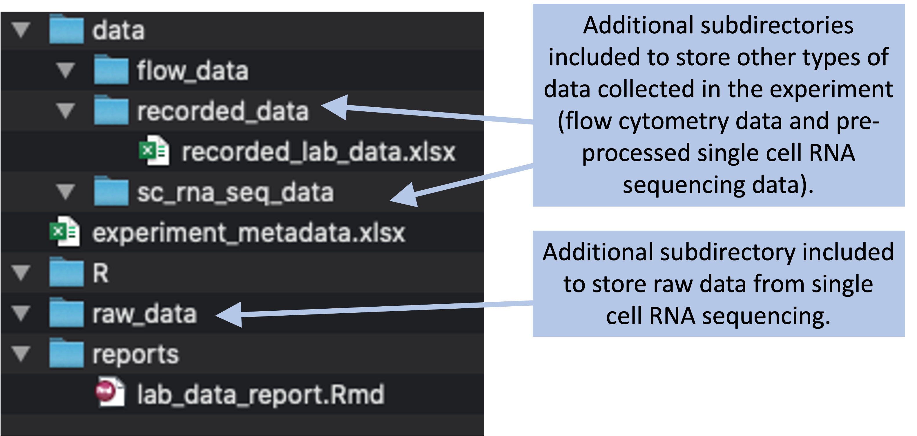
Figure 8.6: Example of a more complex project directory structure that could be created, with directories added to store data collected through flow cytometry and single cell RNA sequencing.

Again, these subdirectories are named in a way that will generalize to many different experiments and yet also clearly labels the contents. Similar subdirectory diversions could also be used within the “raw_data” subdirectory, which would include files for data that need to be pre-processed before they’re used in statistical analysis (modules 12–14). For example, the raw flow cytometry data will need to be gated—a process that will quantify immune cell phenotypes in each sample—before it’s used in statistical analysis.

The exact combination of subdirectories within the “data” subdirectory might change from experiment to experiment. For example, some experiments might include single-cell RNA sequencing assays, while some may not. When we use the template, it will be easy to delete any “data” subdirectories for assays we are not conducting, but by including them in the template, we can insure that we use a consistent name for each subdirectory when we do include it. If you’re trying to be consistent, it’s easier to start with everything you might need and delete some elements to customize for a particular project rather than starting with a minimal framework and adding.

8.4 Step 3: Establishing file name conventions

Next, we decided on how we’d name files in the directory. First, there are some files that will be included in every project. These include a file to record metadata about the experiment, as well as a file to record mouse weights over the course of the experiment and bacterial load at the end of the experiment.

For both of these files, we selected filenames that would balance generalizability with discoverability (see module 7 for more on setting rules for filenames based on these principles). The file with experimental data, for example, is named “experiment_metadata.xlsx”. This name is generic enough that it will work for each of the studies, but it is also clear enough that people will have a good idea of what’s in the file when they explore the project directory. Similarly, the file for recording weights and bacterial load is named “recorded_lab_data.xlsx”, which again balances considerations generalizability with discoverability.

You may have noticed that both these names avoid any special characters, including spaces. Instead, the filenames use underscores to help distinguish different words in the filenames and make them easy to read.

These experiments may have read-outs from laboratory equipment. Examples include data from assays like flow cytometry and single-cell RNA sequencing. In these cases, we’ll keep the filenames that are generated by the laboratory equipment, so that we’ll maintain those standard formats.

8.5 Step 4: Designing data collection templates

The next step is to create any necessary data collection templates. We’ll create a separate spreadsheet for each type of data, but we can group them into files if we’d like (e.g., one spreadsheet file with several separate sheets). In our example, we created two files to store this type of data, one for the metadata that are recorded at the start of the experiment (overall experiment details and the details of each tested treatment) and one for the data that are collected over the course of the experiment (mouse weights and bacterial loads). Within each file, we’ve used separate sheets to record the different types of data. This allows us to keep similar types of data together in the same file, while having a tidy collection format for each specific type of data (Figure 8.7).

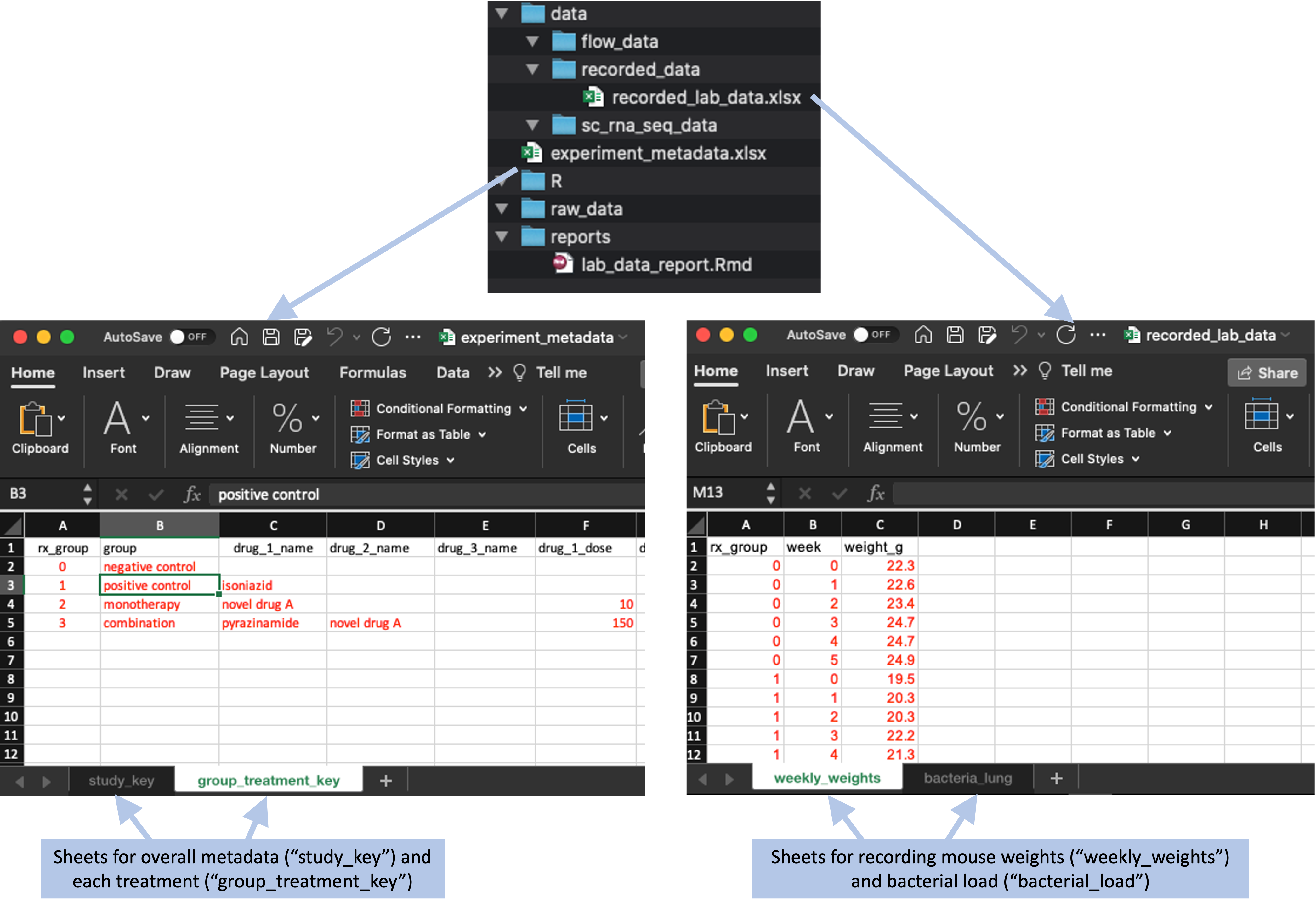
Figure 8.7: Data collection templates for the example project directory template. These templates were created in two files, one for metadata, which is saved in the main directory of the project, and one for data collected in the laboratory during the experiment, which is saved in the ‘data’ subdirectory. Each file is saved as a spreadsheet file, with two sheets in each file to store different types of data.

All of these data collection files are designed using the principles of tidy data collection. In modules 4 and 5, we showed how you can create tidy data collection templates to use, and how these can be paired with reproducible reporting tools to separate the steps of data collection and reporting (modules ?? through 20 go into much more depth on these reproducible reporting tools). Once you have decided on the types of data that you will usually collect for the type of study that this template is for, you can use that process to create tidy data collection templates for each type of data.

When we created the template for each type of data, we added placeholder data (formatted in red to indicate that it is placeholder, rather than final data). This is so the researcher can see an example of how to enter data in the template when they start a new project.

Figure 8.8 gives an example of this process. One of the files that is included in the example template directory shown earlier is a spreadsheet to record metadata on the experiment. This spreadsheet file has two sheets, one that records overall metadata on the study (for example, the weeks of treatment given and the strain of mouse used) and one that records details on each of the treatments that was tested. In the file in the template directory, these spreadsheet pages include placeholder data. These are formatted in red, so that they visually can be identified as placeholders. By including these placeholder data, the researcher can see an example of the format that you expect to be used in recording data in this file. Once the project template is copied, the researcher will replace these data with the real data, and then change the font color to black to indicate that the placeholder data have been replaced (Figure 8.8).

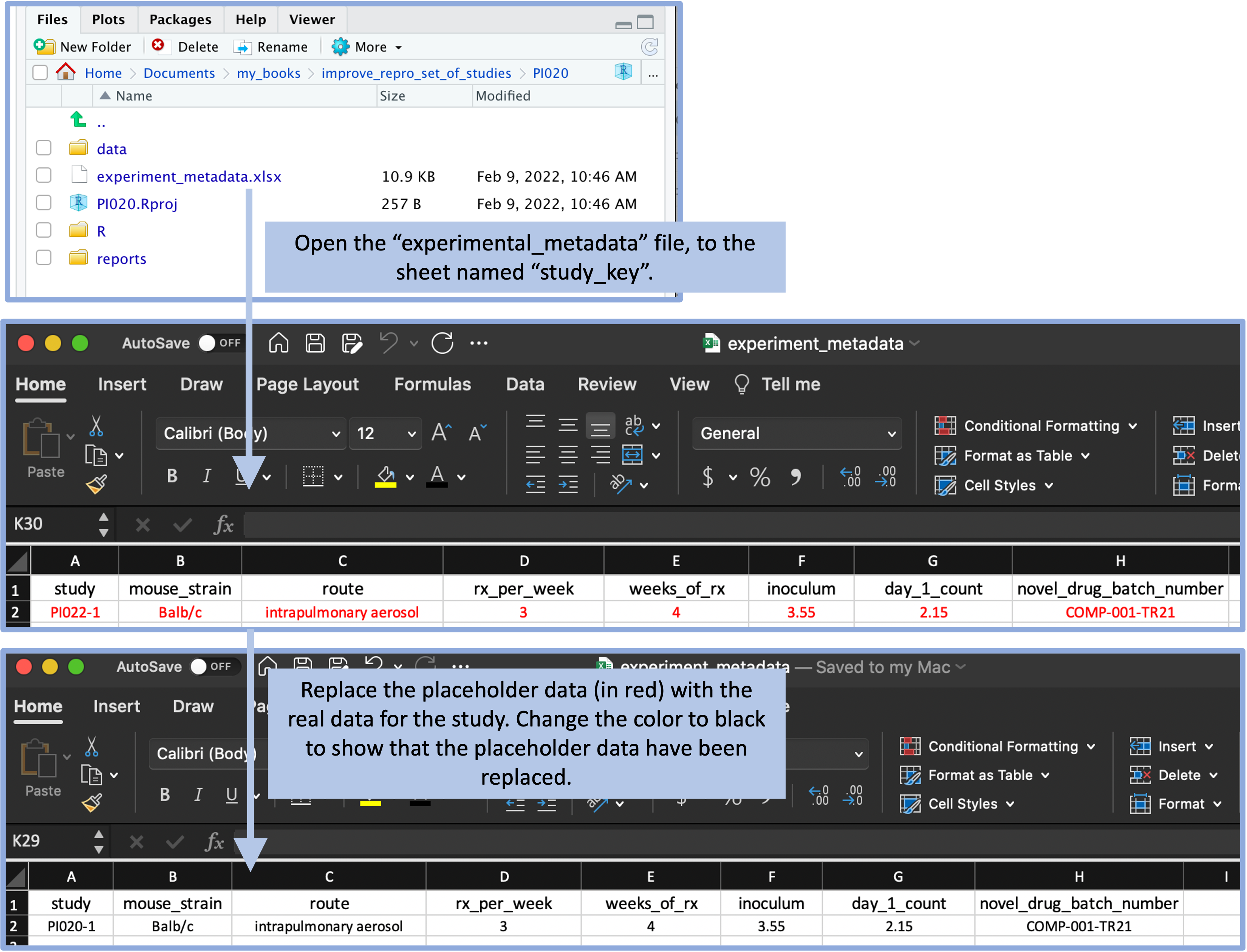
Figure 8.8: The template includes a file with experiment metadata, with a sheet for recording the overall details of the experiment. A user can open this file and replace the placeholder values (in red) with real values for the experiment. By changing the text color to black, the user can have a visual confirmation that the placeholder data have been replaced with real study data.

Another sheet of this spreadsheet allows the researcher to record the details of each of the treatments that were tested in the experiment. Again, placeholder data are included in the template in a red font to help show the researcher how to record the data, and these are meant to be replaced with real data from the specific experiment (Figure 8.9). A similar format is used in the template file to record data from the experiment, including the weights of each animal over each week of treatment and the final bacterial load in each animal at the end of treatment. Again, there are placeholder values in the template file, which the researcher will replace with real data after copying the project template for a new experiment.

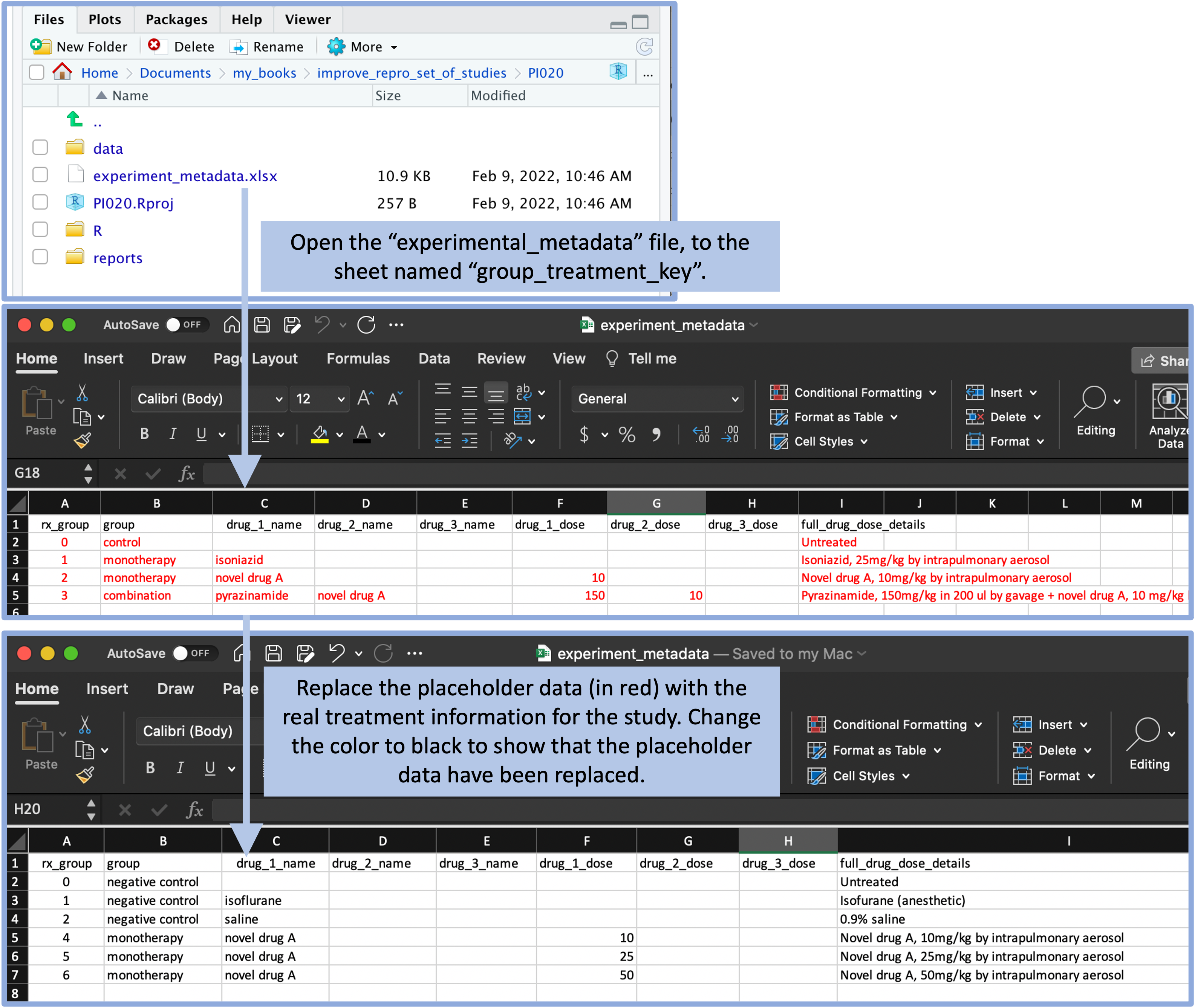
Figure 8.9: The template includes a file with experiment metadata, with a sheet for recording the details of each treatment. A user can open this file and replace the placeholder values (in red) with real values for the treatments in the experiment. By changing the text color to black, the user can have a visual confirmation that the placeholder data have been replaced with real study data.

8.6 Step 5: Designing a report template

A final and optional step is to create one or more template reports. You can create report templates using tools for reproducible reports—in R, a key tool for this is RMarkdown. Here, we’ll cover using this tool for creating a report briefly, but there are many more details in modules 18 through 20. Having example files will help you to develop a template project report that can input the type of data that you typically collect for this type of project.

We created an Rmarkdown file that does this analysis and visualization and included it in the project template directory. This means that the report file will be copied and available each time someone copies the project template directory at the start of a new project. However, you are not obligated to keep the report identical to the template. Instead, the template report serves as a starting point, and you can add to it or adapt it as you work on a study.

This file is created using the RMarkdown format, which combines text with executable code. You can create this template so that it inputs the experimental data from the file formats created for the data recording files in the project template. By doing this, the researcher should be able to “knit” this report for a new experiment, and it should recreate the report based on the data recorded for that experiment (Figure 8.10). By knitting this template report, you can create a nicely formatted version of the report for the experimental data (Figure 8.11).

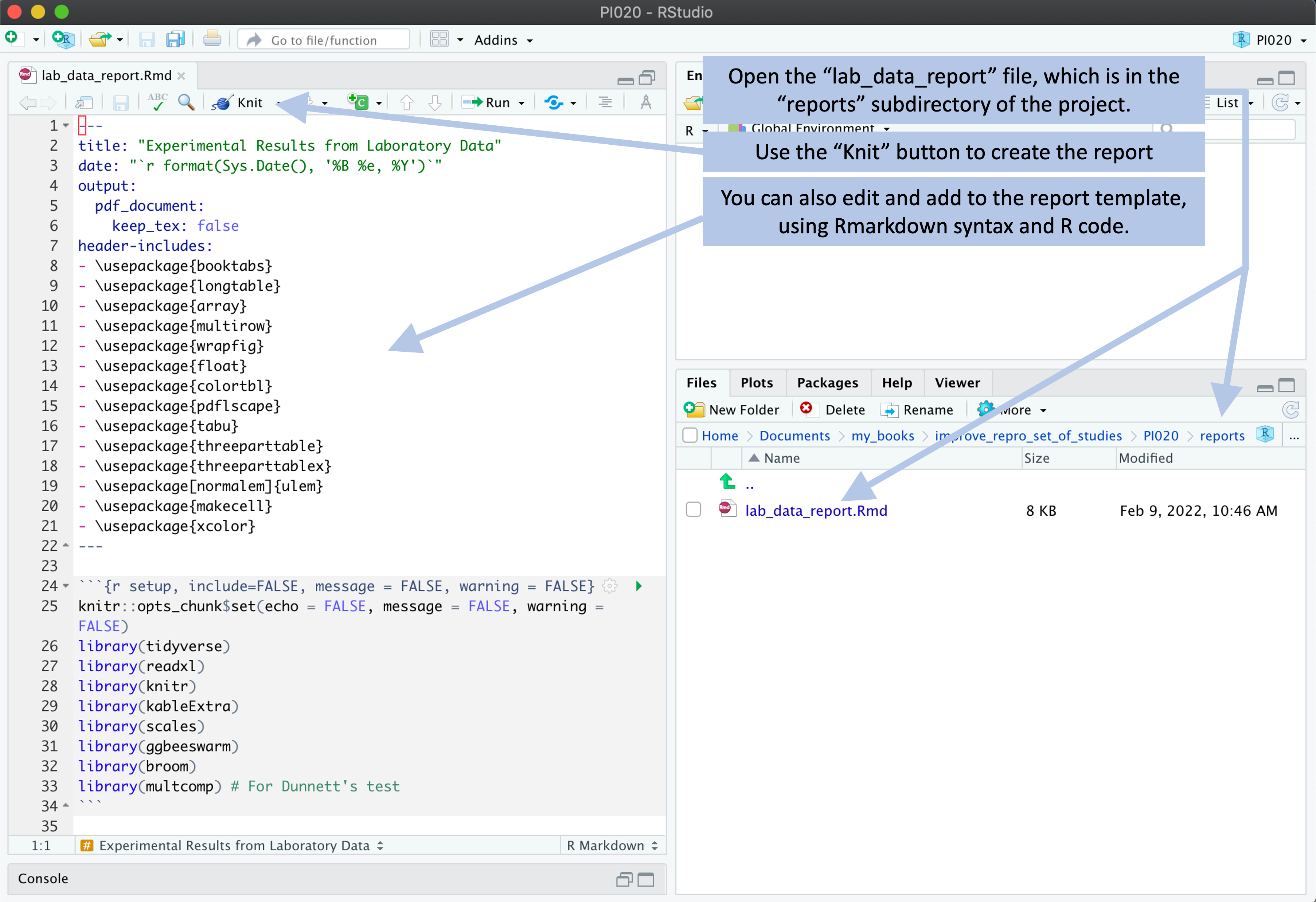
Figure 8.10: Example of how a user can create a report from the template. The template includes an example report, which is written using RMarkdown. The user can open this template report file and use the ‘Knit’ button in RStudio to render the file. As long as the experimental data are recorded using the data template files, the code for this report can process the data to generate a report from the data. The user can also make changes and additions to the template report.

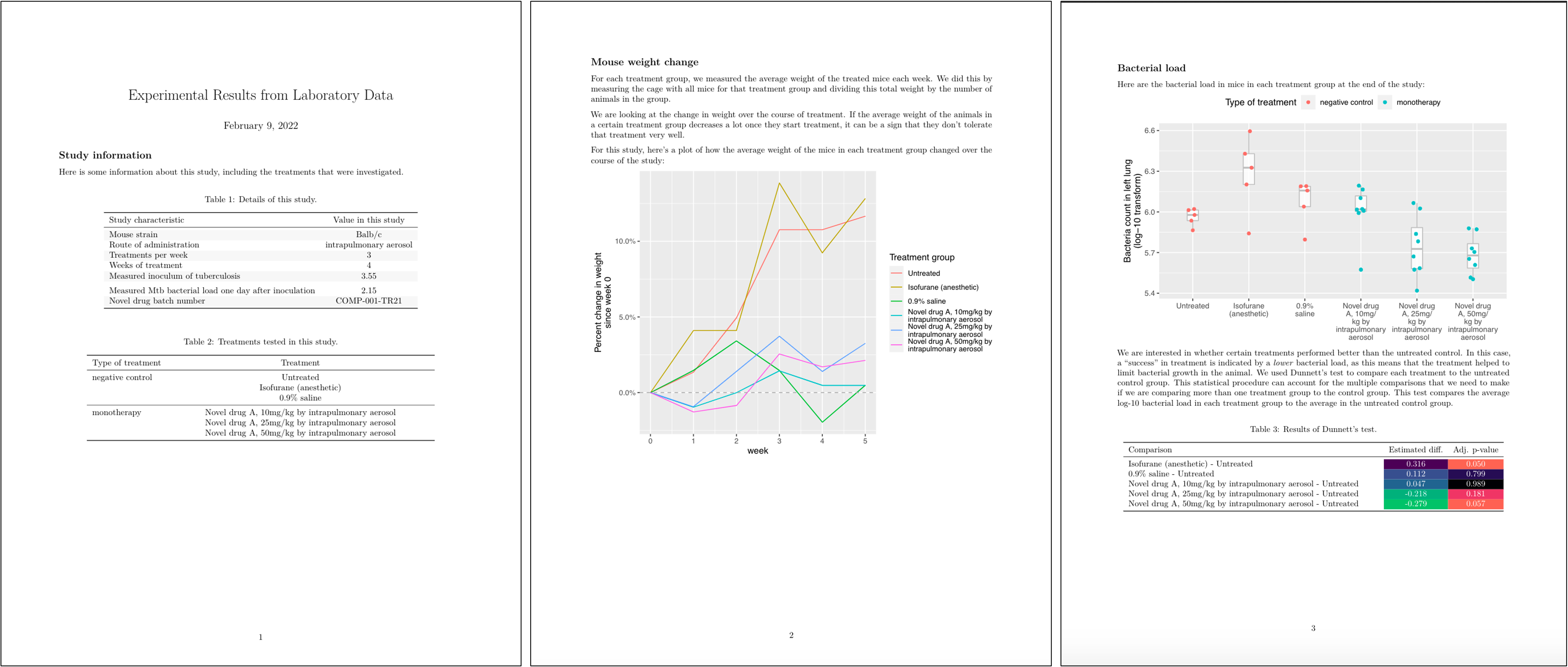
Figure 8.11: Example of the output from ‘knitting’ a report from the project template

Specifically, for this set of studies a preliminary report was designed, with an example shown in Figure 8.12. This report uses the first page to provide a nicely format version of the metadata for the study, including a table with overall details and a table with details for each specific treatment that was tested. The second page provides a graph that shows the percent weight change for mice in each treatment group compared to the weight of that group at the start of treatment. The third page provides a graph that shows the bacterial loads in each mouse, grouped by treatment, as well as the results of running a statistical test, for each treatment group, of the hypothesis that the mean of a transformed version of the measure of bacterial load (log-10) for the group was the same as for the untreated control group.

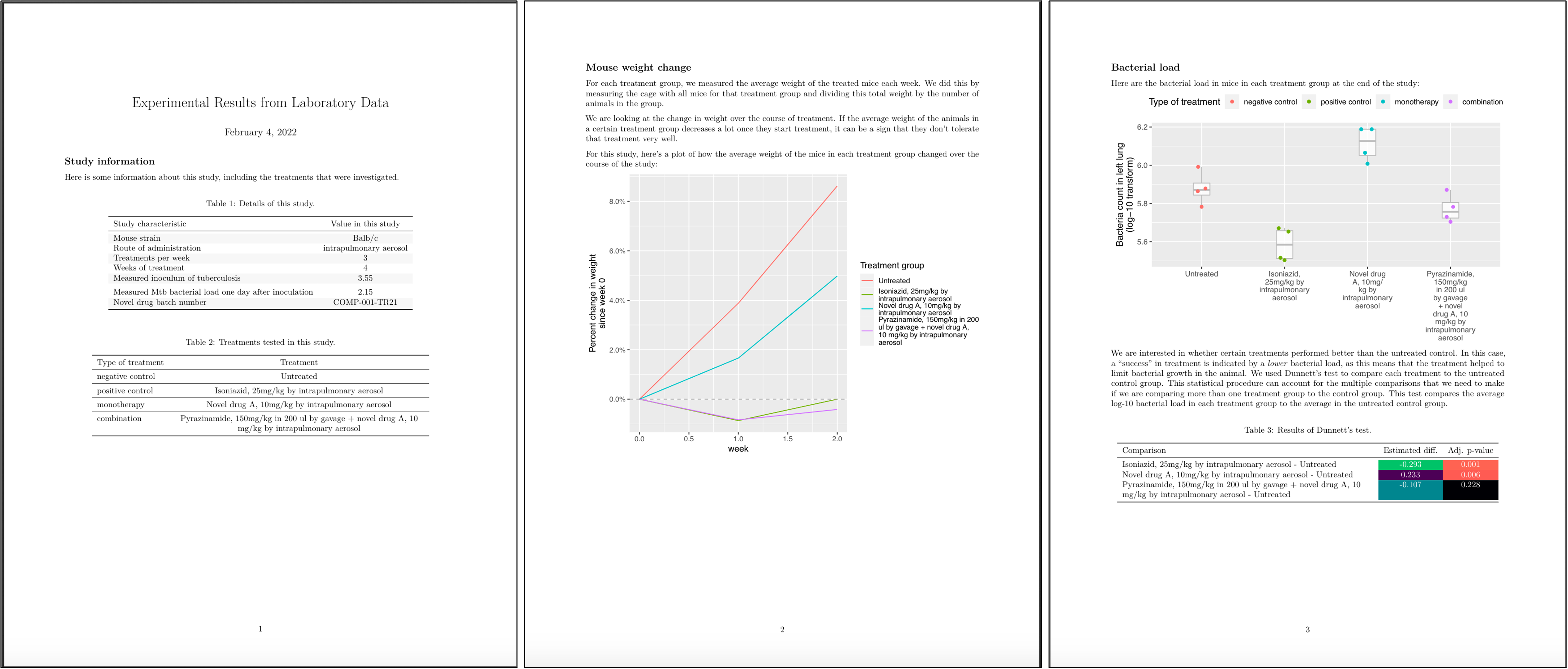
Figure 8.12: Example of the preliminary report generated for each study in the set of example studies for this module. The first page includes metadata on the study, as well as details on each treatment that was tested. The second page shows how mouse weights in each treatment group changed over the course of treatment, to help identify if a treatment was well-tolerated. The third page graphs the bacterial load in each mouse, grouped by treatment, and gives the result of a statistical analysis to test which treatment groups had outcomes that were significantly different from the untreated control group.

Let’s take a closer look at a few of these elements. For example, Figure 8.13 shows the tables from the first page of the report shown in Figure 8.12. If you look back to the data collection for this study (e.g., Figures 8.1 and 8.2), you can see that all of the information in these tables was pulled from data recorded at the start of the study.

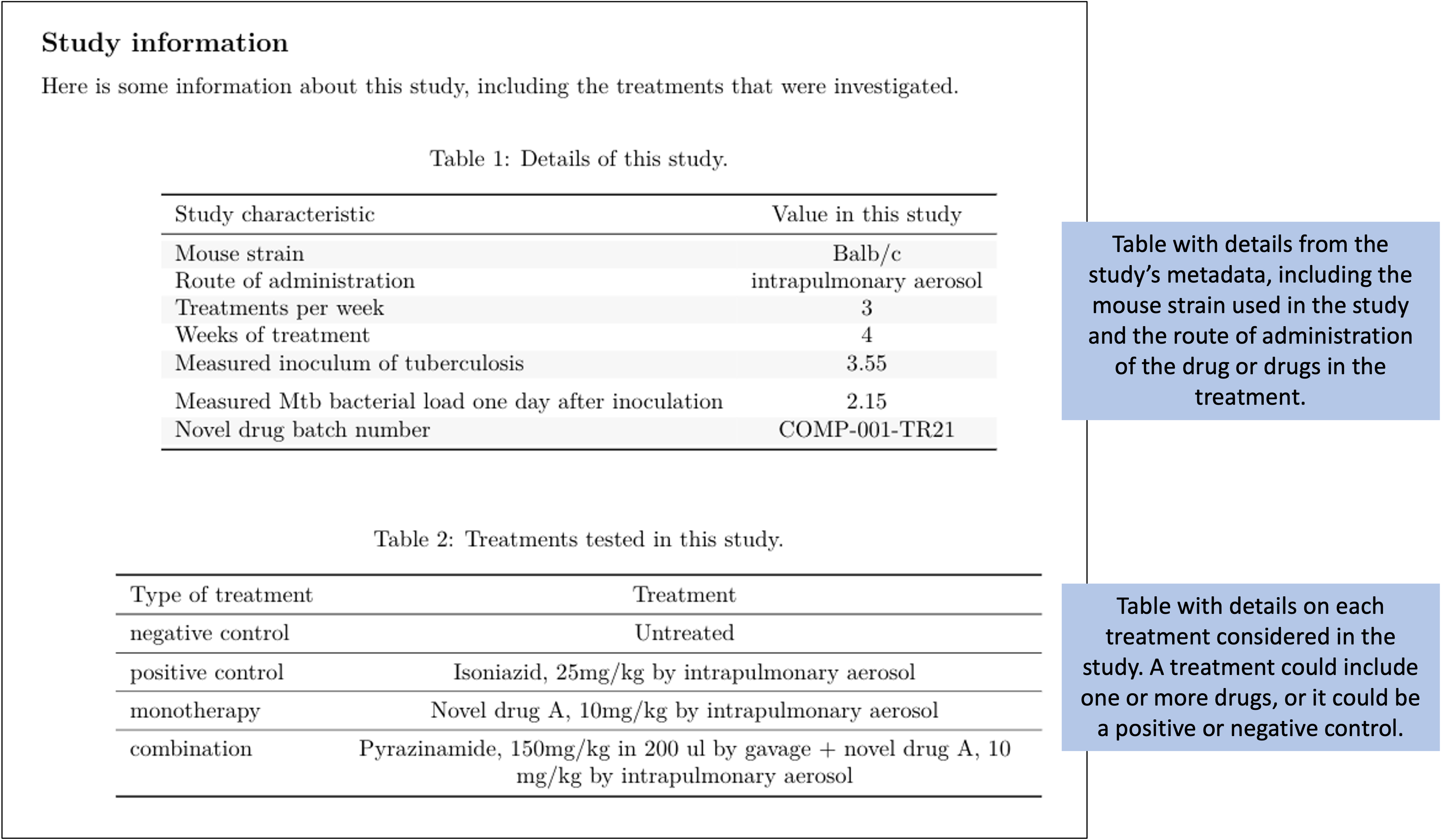
Figure 8.13: Example of one element of the preliminary report generated for each study in the set of example studies for this module. The first page provides tables with metadata about the study and details about each treatment that was tested.

Figure 8.14 shows the second page of the report. This figure has taken the mouse weights—which were recorded in one of the data collection templates for the project (Figure 8.3)—and used them to generate a plot of how average mouse weight in each treatment group changed over the course of the treatment.

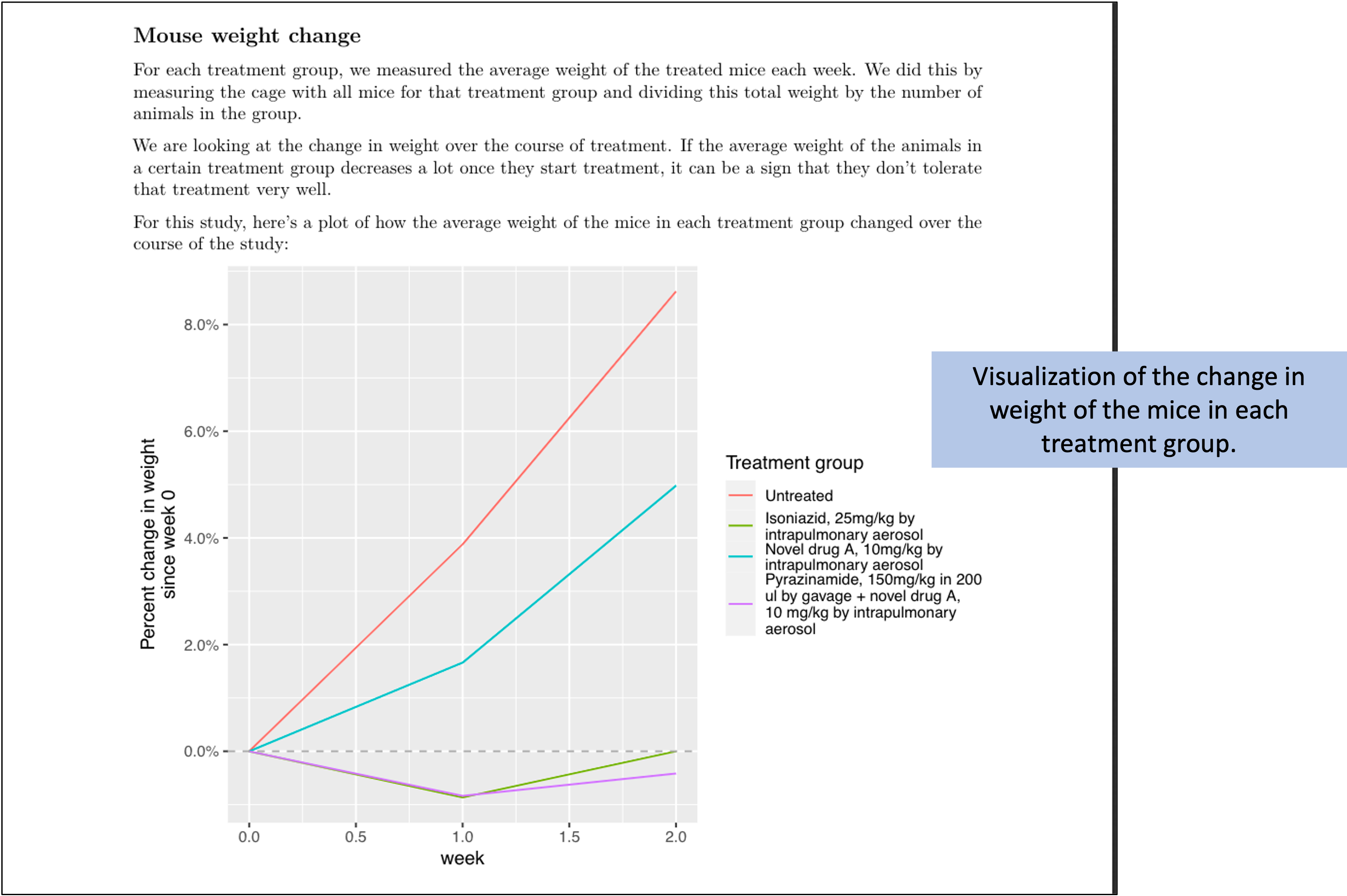
Figure 8.14: Example of one element of the preliminary report generated for each study in the set of example studies for this module. The second page provides a plot of how the weights of mice in each treatment changed over the course of treatment.

Figure 8.15 shows the last page of the report. This page starts with a figure that shows the bacterial load in the lungs of each mouse in the study at the end of the treatment period. In this figure, the measurement for each mouse is shown with a point, and these points are grouped by the treatment group of the mouse. Boxplots are added to show the distribution across the mice in each group. The color is used to show whether the treatment was a negative control, a positive control, a monotherapy, or a combined therapy. The second part of the page gives a table with the results from running a statistical analysis to compare the bacterial load for mice in each treatment group to the bacterial load in the mice in the untreated control group. Color is added to the table to highlight treatments that had a large difference in bacterial load from the untreated control, as well as treatments for which the difference from the untreated control was estimated to be statistically significant. All the data for these results, including the labels for the plot, are from the data collected in the data collection templates shown earlier.

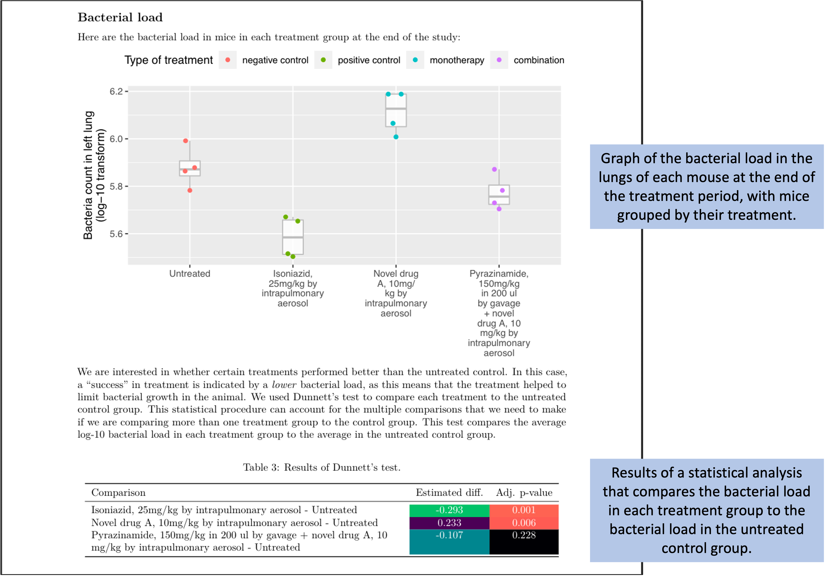
Figure 8.15: Example of one element of the preliminary report generated for each study in the set of example studies for this module. The third page provides results on how bacterial load in the lungs compares among treatments at the end of the treatment period.

We wrote the code in the report in a way that it will still run if there are more or fewer observations in any of the data collection files, so the report template has some flexibility in terms of how each study in the set of studies might vary. For example, in the example set of studies, some of the experiments were run using only a control group of mice, while others were run to test several different treatment groups. The report template can accommodate these differences across studies in the set of studies.