3.9 RMarkdown for creating reproducible data pre-processing protocols
The R extension package RMarkdown can be used to create documents that combine code and text in a ‘knitted’ document, and it has become a popular tool for improving the computational reproducibility and efficiency of the data analysis stage of research. This tool can also be used earlier in the research process, however, to improve reproducibility of pre-processing steps. In this module, we will provide detailed instructions on how to use RMarkdown in RStudio to create documents that combine code and text. We will show how an RMarkdown document describing a data pre-processing protocol can be used to efficiently apply the same data pre-processing steps to different sets of raw data.
Objectives. After this module, the trainee will be able to:
- Define RMarkdown and the documents it can create
- Explain how RMarkdown can be used to improve the reproducibility of research projects at the data pre-processing phase
- Create a document in RStudio using RMarkdown
- Apply it to several different datasets with the same format
3.9.1 Creating knitted documents in R
In the last module, we described what knitted documents are, as well as the advantages of using knitted documents to create data pre-processing protocols for common pre-processing tasks in your research group. In this module, we will go into more detail about how you can create these documents using R and RStudio, and in the next module we will walk through an example data pre-processing protocol created using this method.
R has a special format for creating knitted documents called Rmarkdown. Later in this module, we will provide details on creating these documents, but first, we will provide some details of some of the specific conventions used in this type of knitted documents. As with other knitted documents, Rmarkdown documents are originally written in plain text. In the previous module, we discussed how knitted documents will use a markup language within the plain text for formatting; for RMarkdown files, the markup language used is Markdown. Since the laguage is Markdown, the preamble for each document uses YAML. We described in the previous module how knitted documents include executable code, along with the formatted text. By default, executable code for RMarkdown files will be in R, but there are also options to include executable code in the document in a number of other programming languages.
3.9.2 Creating and exploring an Rmarkdown file
Creating a new Rmarkdown file and exploring the template.
First, we will explain how you can create a new Rmarkdown document using RStudio. Like other plain text documents, an Rmarkdown file should be edited using a text editor, rather than a word processor like Word or Google Docs. It is easiest to use the Rstudio IDE as the text editor when creating and editing an R markdown document, as this IDE has incorporated some helpful functionality for working with plain text documents for Rmarkdown. The RStudio IDE can be downloaded and installed as a free software, as long as you use the personal version (RStudio creates higher-powered versions for corporate use). Since RStudio is free and has many helpful tools for working with Rmarkdown, we will focus on using this interface in our advice in this module.
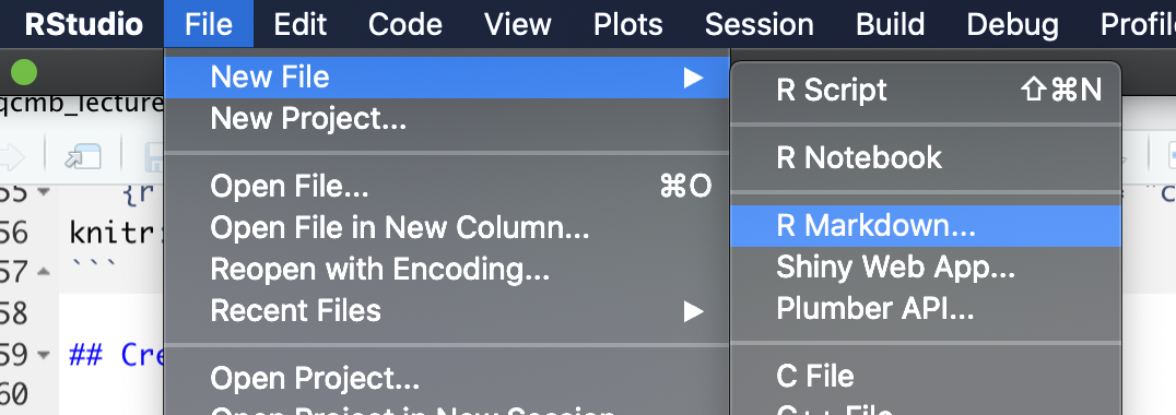
In RStudio, you can create a number of types of new files through the “File” menu. To create a new R markdown file, choose “New File” and then choose “Rmarkdown” from the choices in that menu. Figure 3.5 shows an example of what this menu option looks like.
Figure 3.5: RStudio pull-down menus to help you navigate to open a new Rmarkdown file.
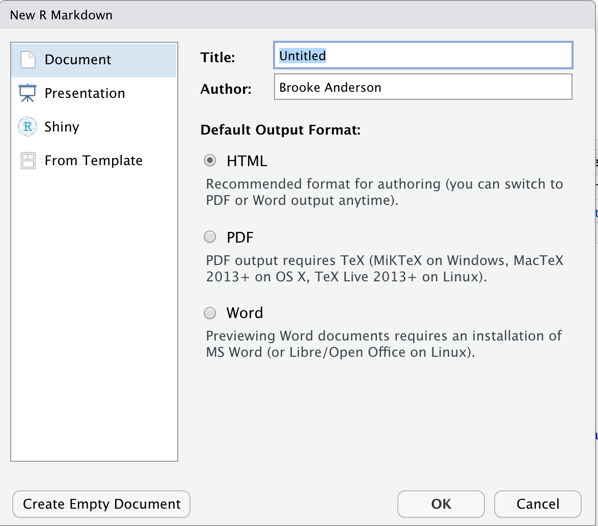
This will open a window with some options you can specify some of the overall information about the document (Figure 3.6), including the title and the author, and you can specify the output format that you would like. Possible output formats include HTML, Word, and PDF. You should be able to use the HTML and Word output formats without any additional software. If you would like to use the PDF output, you will need to install one other piece of software: Miktex for Windows, MacTex for Mac, or TeX Live for Linux. These are all pieces of software with an underlying TeX engine and all are open-source and free.
Figure 3.6: Options available when you create a new Rmarkdown file in RStudio. You can specify information that will go into the document’s preamble, including the title and authors and the format that the document will be output to (HTML, Word, or PDF).
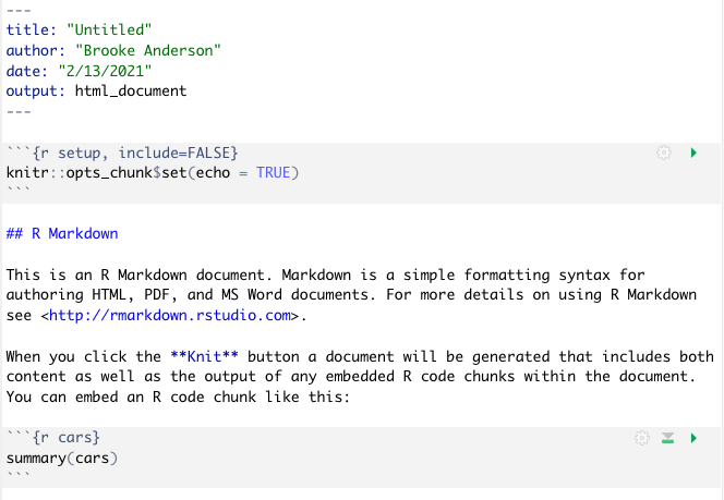
Once you have selected the options in this menu you can choose the “Okay” button (Figure 3.6). This will open a new document. This document, however, won’t be blank. Instead it will include an example document written in Rmarkdown (Figure 3.7). This example document helps you navigate how the Rmarkdown process works, by letting you test out a sample document. It also gives you a starting point—once you understand how the example document works, you can edit it and change it to convert it into the document you would like to create.
Figure 3.7: Example of the template Rmarkdown document that you will see when you create a new Rmarkdown file in RStudio. You can explore this template and try rendering (knitting) it. Once you are familiar with how this example works, you can edit the text and code to adapt it for your own document.
If you have not used Rmarkdown before, it is very helpful to try knitting this example document before making changes, to explore how pieces in the document align with elements in the rendered output document. Once you are familiar with the line-up between elements in this file in the output document, you delete parts of the example file and insert your own text and code.
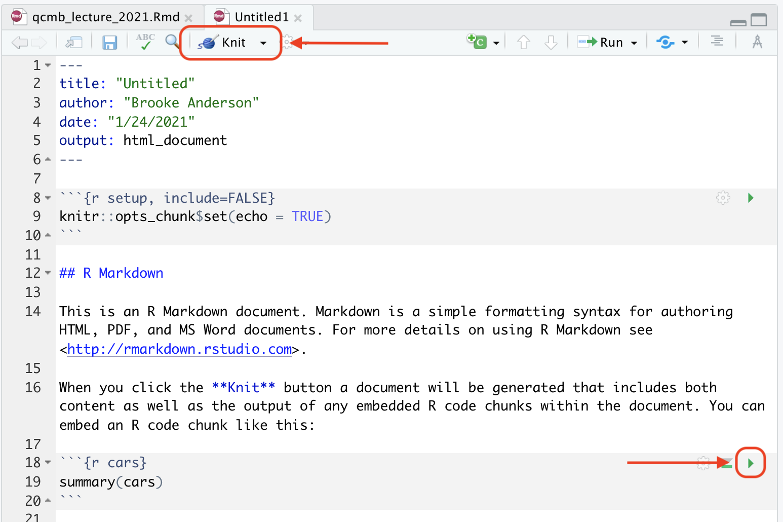
We will walk you through exploring this example document, as well as aligning it with the formatted output document (Figure 3.8). First, to render this or any Rmarkdown document, if you are in RStudio you can use the “Knit” button at the top of the file, as shown in Figure 3.9. When you click on this button, it will render the entire document to the output format you’ve selected (HTML, PDF, or Word). This rendering process will both run the executable code and apply all formatting. The final output (Figure 3.8, right) will pop up in a new window. As you start with Rmarkdown, it is useful to look at this output to see how it compares with the plain text Rmarkdown file (Figure 3.8, left).
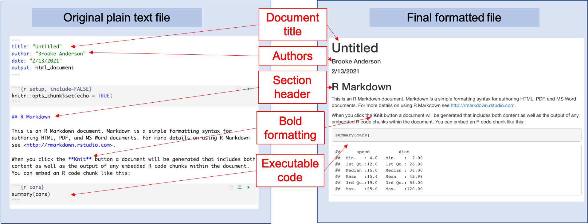
Figure 3.8: Example of the template Rmarkdown document that you will see when you create a new Rmarkdown file in RStudio. You can explore this template and try rendering (knitting) it. Once you are familiar with how this example works, you can edit the text and code to adapt it for your own document.
Figure 3.9: Example of the template Rmarkdown document, highlighting buttons in RStudio that you can use to facilitate working with the document. The ‘knit’ button, highlighted at the top of the figure, will render the entire document. The green arrow, highlighted lower in the figure within a code chunk, can be used to run the code in that specific code chunk.
You will also notice, after you first render the document, that your working directory has a new file with this output document. For example, if you are working to create an HTML document using an Rmarkdown file called “my_report.Rmd,” once you knit your Rmarkdown file, you will notice a new file in your working directory called “my_report.html.” This new file is your output file, the one that you would share with colleagues as a report. You should consider this output document to be read only—in other words, you can read and share this document, but you should not make any changes directly to this document, since they will be overwritten anytime you re-render the original Rmarkdown document.
Next, let’s compare the example Rmarkdown document (the one that is given when you first open an Rmarkdown file in RStudio) with the output file that is created when you render this example document (Figure 3.8). If you look at the output document (Figure 3.8, right), you can notice how different elements align with pieces in the original Rmarkdown file (Figure 3.8). For example, the output document includes a header with the text “R Markdown.” This second-level header is created by the Markdown notation in the original file of:
## R MarkdownThis header is formatted in a larger font than other text, and on a separate
line—the exact formatting is specified within the style file for the Rmarkdown
document, and will be applied to all second-level headers in the document. You
can also see formatting specified through things like bold font for the word
“Knit,” through the Markdown syntax **Knit**, and a clickable link specified
through the syntax <http://rmarkdown.rstudio.com>. At the beginning of the
original document, you can see how elements like the title, author, date, and
output format are specified in the YAML. Finally, you can see that special
character combinations demarcate sections of executable code.
Formatting text with Markdown.
For the main text in an Rmarkdown document, all formatting is done using Markdown as the markup language. Markdown is a popular markup language, in part because it is a good bit simpler than other markup languages like HTML or LaTeX. This simplicity means that it is not quite as expressive as other markup languages. However, Markdown provides adequate formatting for 90% of the formatting you will typically want to do for a research report or pre-processeing protocol, and by staying simpler, it is much easier to learn the Markdown syntax quickly compared to other markup languages.
As with other markup languages, Markdown uses special characters or combinations of characters to indicate formatting within the plain text of the original document. When the document is rendered, these markings are used by the software to create the formatting that you have specified in the final output document. Some example formatting symbols and conventions for Markdown include:
- to format a word or phrase in bold, surround it with two asterisks (
**) - to format a word or phrase in italics, surround it with one asterisk (
*) - to create a first-level header, put the header text on its own line, starting the line with
# - to create a second-level header, put the header text on its own line, starting the line with
## - separate paragraphs with empty lines
- use hyphens to create bulleted lists
One thing to keep in mind when using Markdown, in terms of formatting, is that
white space can be very important in specifying the formatting. For example when
you specify a new paragraph, you must leave a blank line from your previous
text. Similarly when you use a hash (#) to indicate a header, you must leave a
blank space after the hash before the word or phrase that you want to be used in
that header. To create a section header, you would write:
# Initial Data InspectionMeanwhile this:
#Initial Data InspectionWould render to:
#Initial Data Inspection
Similarly, white space is needed to separate paragraphs. For example, this would create two paragraphs:
This is a first paragraph.

This is a second.
Meanwhile this would create one:
This is a first paragraph.
This is still part of the first paragraph.
The syntax of Markdown is fairly simple and can be learned quickly. For more details on this syntax, you can refer to the Rmarkdown reference guide at https://rstudio.com/wp-content/uploads/2015/03/rmarkdown-reference.pdf. The basic formatting rules for Markdown are also covered any number of more extensive resources for Rmarkdown that we will point you to later in this module.
Creating a preamble with YAML.
In the previous module, we explained how knitted documents include a preamble to specify some metadata about the document, including elements like the title, authors, and output format. In R, this preamble is created using YAML. In this subsection, we provide some more details on using this YAML section in Rmarkdown documents.
When you initially create an Rmarkdown document, you select the output format
for it (e.g., pdf, Word, HTML). You can change this output selection once you’ve
created the document, however, by making a change in a special section at the
top of the RMarkdown document called the “YAML.” The YAML is a special section
at the top of an RMarkdown document (the original, plain text file, not the
rendered version). It is set off from the rest of the document using a special
combination of characters, using a process very similar to how executable code
is set off from other text with a special set of characters so it can be easily
identified by the software program that renders the document. For the YAML, this
combination of characters is three hyphens (---) on a line by themselves to
start the YAML section and then another three on a line by themselves to end it.
Here is an example of what the YAML might look like at the top of an RMarkdown
document:
---
title: "Laboratory report for example project"
author: "Brooke Anderson"
date: "1/12/2020"
output: word_document
---
Within the YAML itself, you can specify different options for your document.
You can change simple things like the title, author, and date, but you can
also change more complex things, including how the output document is rendered.
For each thing that you want to specify, you specify it with a special
keyword for that option and then a valid choice for that keyword. The idea
is very similar to setting parameter values in a function call in R. For
example, the title: keyword is a valid one in RMarkdown YAML. It allows you
to set the words that will be printed in the title space, using title formatting,
in your output document. It can take any string of characters, so you can put in
any text for the title that you’d like, as long as you surround it with quotation
marks. The author: and date: keywords work in similar ways. The output:
keyword allows you to specify the output that the document should be rendered to.
In this case, the keyword can only take one of a few set values, including
word_document to output a Word document, pdf_document to output a pdf
document (see later in this section for some more set-up required to make that
work), and html_document to output an HTML document.
As you start using RMarkdown, you will be able to do a lot without messing with the YAML much. In fact, you can get a long way without ever changing the values in the YAML from the default values they are given when you first create an RMarkdown document. As you become more familiar with R, you may want to learn more about how the YAML works and how you can use it to customize your document—it turns out that quite a lot can be set in the YAML to do very interesting customizations in your final rendered document. The book R Markdown: The Definitive Guide [ref], which is available free online, has sections discussing YAML choices for both HTML and pdf output, at https://bookdown.org/yihui/rmarkdown/html-document.html and https://bookdown.org/yihui/rmarkdown/pdf-document.html, respectively. There is also a talk that Yihui Xie, the creator of RMarkdown, gave on this topic at a past RStudio conference, available at https://rstudio.com/resources/rstudioconf-2017/customizing-extending-r-markdown/.
Executable code in Rmarkdown files.
In the previous module, we described how knitted documents use special markers to indicate where sections of executable code start and stop. In RMarkdown, the markers you will use to indicate executable code look like this:
```r{}
my_object <- c(1, 2, 3)
```
The first part of this marker (```{r}) indicates that a section of
code is starting. Then end part (```) indicates that the file is
moving back to regular Markdown. In the first marker, you can use the simplest
form (```{r}) to indicate the start of the code. However, you can also
include options to customize actions when the code in that section is executed.
There are many options that you can set for each code chunk. These options will
specify how the code in that section of executable code will be run and how the
output from running the code will be presented. These specifications are called
chunk options, and you specify them in the special character combination
where you mark the start of executable code. For example, you can specify that
the code should be printed in the document, but not executed, by setting the
eval parameter to FALSE with ```{r eval = FALSE} as the marker to
start the code section.
The chunk options also include echo, which can be used to specify whether to
print the code in that code chunk when the document is rendered. For some
documents, it is useful to print out the code that is executed, where for other
documents you may not want that printed. For example, for a pre-processing
protocol, you are aiming to show yourself and others how the pre-processing was
done. In this case, it is very helpful to print out all of the code, so that
future researchers who read that protocol can clearly see each step. By
contrast, if you are using Rmarkdown to create a report or an article that is
focused on the results of your analysis, it may make more sense to instead hide
the code in the final document.
As part of the code options, you can also specify whether messages and warnings created when running the code should be included in the document output, and there are number of code chunk options that specify how tables and figures rendered by the code should be shown. For more details on the possible options that can be specified for how code is evaluated within an executable chunk of code, you refer to the Rmarkdown cheat sheet available at https://rstudio.com/wp-content/uploads/2015/02/rmarkdown-cheatsheet.pdf
RStudio has some functionality that is useful when you are working with code in Rmarkdown documents. Within each code chuck are some buttons that can be used to test out the code in that chunk of executable code. One is the green right arrow key to the right at the top of the code chunk, highlighted in Figure 3.9. This button will run all of the code in that chunk and show you the output in an output field that will open directly below the code chunk. This functionality allows you to explore the code in your document as you build it, rather than waiting until you are ready to render the entire document. The button directly to the left of that button, which looks like an upward-pointing arrow over a rectangle, will execute all code that comes before this chunk in the document. This can be very helpful in making sure that you have set up your environment to run this particular chunk of code.
3.9.3 More advanced Rmarkdown functionality
The details and resources that we have covered so far focus on the basics of Rmarkdown. You can get a lot done just with these basics. However, the Rmarkdown system is very rich and allows complex functionality beyond these basics. In this subsection, we will highlight just a few of the ways Rmarkdown can be used in a more advanced way. Since this topic is so broad, we will focus on elements that we have found to be particularly useful for biomedical researchers as they become more advanced Rmarkdown users. For the most part, we will not go into extensive detail about how to use these more advanced features in this module, but instead point to resources where you can learn more as you are ready. If you are just learning Rmarkdown, at this point it will be helpful to just know that some of these advanced features are available, so you can come back and explore them when you become familiar with the basics. However, we will provide more details for two elements that we find particularly useful in creating data pre-processing protocols: including bibliographical references and including mathematical equations. In the next module, we walk through an example of using RMarkdown, and in this example we show how you can use these two more advanced features when creating a pre-processing protocol.
Including bibliographical references.
You can use Rmarkdown, in combination with something called BibTeX, as a referencing system. This allows you to include bibliographical references in the documents that you create, and Rmarkdown will handle the creation of the references section and the numbering of the documents within your text.
To include references in RMarkdown documents, you can use something called BibTeX. This has three components:
- Create a plain text file with listings for each of
your references (BibTeX file). Save it with the
extension
.bib. - In your RMarkdown document, include the filepath to this BibTeX file.
- In the text of the RMarkdown file, include a key and special character combination anytime you want to reference a paper.
Once you have a BibTeX file, you will include its path in the YAML:
  ---
  title: "Reproducible Research with R"
  author: "Brooke Anderson"
  date: "1/25/2021"
  output: beamer_presentation
  bibliography: mybibliography.bib
  ---
It is easiest if you save the BibTeX file in the same directory as the RMarkdown document.
You can add references in the text using a key for each paper
within special characters ([@paper1, @paper2]).
For example, you would write:
This technique follows earlier work [@fox2020,
@anderson2019].
To create:
``This technique follows earlier work (Fox et al. 2020, Anderson et al. 2019)."
With full paper details included at the end of the document.
Put all the bibliographical details in the BibTeX file:
You will have a file named something like mybibliography.bib
with entries for each paper like this:
@article{fox2020,
  title={Cyto-feature engineering: A pipeline for flow cytometry
    analysis to uncover immune populations and associations with
    disease},
  author={Fox, Amy and Dutt, Taru S and Karger, Burton and Rojas,
    Mauricio and Obreg{\'o}n-Henao, Andr{\'e}s and
    Anderson, G Brooke and Henao-Tamayo, Marcela},
  journal={Scientific Reports},
  volume={10},
  number={1},
  pages={1--12},
  year={2020}
}
You can get these details from Google Scholar:
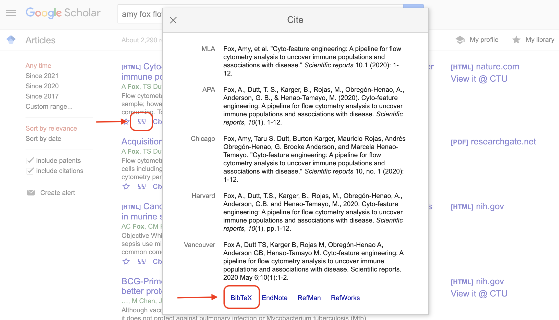
Figure 3.10: Example of using Google Scholar to get bibliographical information for a BibTeX file. When you look up an article on Google Scholar, there is an option (the quotation mark icon under the article listing) to open a pop-up window with bibliographical information. At the bottom of this pop-up box, you can click on ‘BibTeX’ to get a plain text version of the BibTeX entry for the article. You can copy and paste this into you BibTeX file.
Including mathematical equations.
Next, you can include mathematical equations within an Rmarkdown document. This allows you to use nice formatting whenever you need to include an equation within your document.
You can include math using a system developed for specifying mathematical equations in LaTeX. [Add more on math]
Including executable code in other languages.
In your RMarkdown documents, you include executable code in special sections (“chunks”) that are separated from the regular text using a special combination of characters, as described earlier in this module and in the previous module. By default, in Rmarkdown files the code in these chunks are executed using the R programming language. However, you can also include executable code in a number of other programming languages. For example, you could set some code chunks to run Python, others to run Julia, and still others (e.g., bash) to run a shell script.
This can be very helpful if you have steps in you Python that use code in different languages. For example, there may be a module in Python that works well for an early step in your data preprocessing, and then later steps that are easier with general R functions. This presents no problem in creating an RMarkdown data pre-processing protocol, as you can include different steps using different languages.
The program that is used to run the code in a specific chunk is called the
“engine” for that chunk [ref—R Markdown def guide]. You can change the engine
by changing the combination of characters you use to demarcate the start of
executable code. When you are including a chunk of R code, you mark it off
starting with the character combination ```{r}. You change this to
give the engine you would like to use—for example, you would include a chunk
of Python code using ```{python} [ref—R Markdown def guide]. When
your RMarkdown document is rendered, your computer will use the specified
software to run each code chunk. Of course, to run that piece of code, your
computer must have that type of software installed and available. For example,
if you include a chunk of code that you’d like to run with a Python engine, you
must have Python on your computer.
While you can use many different software programs as the engine for each code chunk, there are a few limitations with some programs. For many open-source software programs, the results from running a chunk of code with that engine will be available for later code chunks that also use that engine to use as an input [ref—R Markdown def guide]. This is not the case, however, for most of the available engines. For example, if you use the SAS software program as the engine for one of your code chunks, the output from running that code will not be available to input to later code in the document.
Caching code results.
Some code can take a while to run, particularly if it is processing very large datasets. By default, RMarkdown will re-run all code in the document every time you render it. This is usually the best set-up, since it allows you to confirm that the code is all executing as desired each time the code is rendered. However, if you have steps that take a long time, this can make it so the RMarkdown document takes a long time to render each time you render it.
To help with this problem, RMarkdown has a system that allows you to cache results from some or all code chunks in the document. This is a really nice system—it will check the inputs to that part of the code each time the document is run. If those inputs have changed, it will take the time to re-run that piece of code, to use the updated inputs. However, if the inputs have not changed since the last time the document was rendered, then the last results for that chunk of code will be pulled from memory and used, without re-running the code in that chunk. This saves time most of the times that you render the document, while taking the time to re-run the code when necessary, because the inputs have changed and so the outputs may be different.
There are some downsides to caching. For example, caching can increase the storage space it takes to save Rmarkdown work, as intermediate results are saved. However, if some of your code is very time-intensive to run, it may make sense to look into caching options with Rmarkdown. For more on caching with Rmarkdown documents, see this section of the R Markdown Cookbook [ref].
Outputting to other formats.
You can use RMarkdown to create documents other than traditional reports. Scientists might find the outputs of presentations and posters particularly useful.
RMarkdown has allowed a pdf slide output for a long time. This output leverages the “beamer” format from LaTeX. You can create a series of presentation slides in RMarkdown, using Markdown to specify formatting, and then the document will be rendered to pdf slides. These slides can be shown using pdf viewer software, like Adobe Acrobat, set either to full screen or to the presentation option. More recently, capability has been added to RMarkdown that allows you to create PowerPoint slides. Again, you will start from an RMarkdown document, using Markdown syntax to do things like divide content into separate slides. Regardless of the output format you choose (pdf slides or PowerPoint), the code to generate figures and tables in the presentation can be included directly in the RMarkdown file, so it is re-run with the latest data each time you render the presentation.
It is also possible to use RMarkdown to create scientific posters, although this
is a bit less common and there are fewer tutorial resources with instructions on
doing this. To find out more about creating scientific posters with Rmarkdown,
you can start by looking at the documentation for some R packages that have been
created for this process. Two include the posterdown package [ref], with
documentation available at
https://reposhub.com/python/miscellaneous/brentthorne-posterdown.html, and the
pagedown package [ref], with documentation available at
https://github.com/rstudio/pagedown. There are also some blog posts available
where researchers describe how they created a poster with Rmarkdown; one
thorough one is “How to make a poster in R” by Wei Yang Tham, available at
https://wytham.rbind.io/post/making-a-poster-in-r/.
This idea of customizing Rmarkdown documents has evolved in another useful way through the idea of Rmarkdown templates. These are templates that are customized—often very highly customized—while allowing you to write the content using Rmarkdown. One area where these templates can be very useful to scientists is with article templates that are customized for specific scientific journals. A number of scientific journals have created LaTeX templates that can be used when writing drafts to submit to the journal. These templates produce a draft that is nicely formatted, following all the journal’s guidelines for submission, and in some cases formatted as the final article would be for the journal. These templates have existed for a long time, particularly for journals in fields in which LaTeX is commonly used for document formatting, including physics and statistics. However, the templates traditionally required you to use LaTeX, which is a complex markup language with a high threshold for learning to use it.
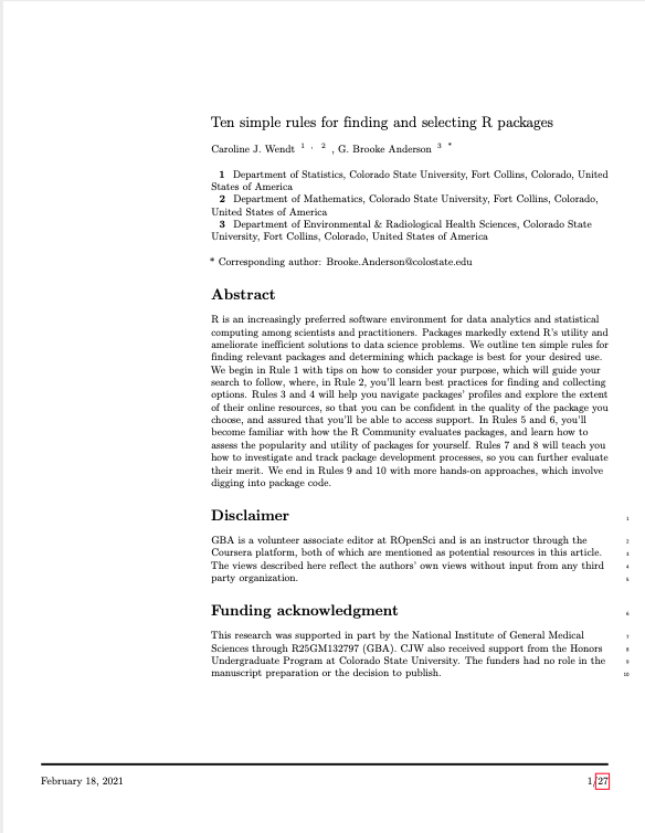
Now, many of these article templates have been wrapped within an Rmarkdown template, allowing you to leverage them while writing all the content in Rmarkdown syntax, and allowing you to include executable code directly in the draft. An example of the first page of an article created in Rmarkdown using one of these article templates is shown in Figure 3.11.
Figure 3.11: Example of a manuscript written in Rmarkdown using a templat. This figure shows the first page of an article written for submission to PLoS Computation Biology, written in Rmarkdown while using the PLoS template from the rticles package. The full article, including the Rmarkdown input and final pdf, are available on GitHub at https://github.com/cjwendt/plos_ten.
These Rmarkdown templates are typically available through R packages, which you
can install on your computer in the same way you would install any R package
(i.e., with the install.packages function). Many journal article templates are
available through the rticles package [ref], including the template used to
create the manuscript shown in Figure 3.11. You can find
more information about the rticles package on its GitHub page, at
https://github.com/rstudio/rticles. There is also a section in the book R
Markdown: A Definitive Guide [ref] on writing manuscripts for scientific
journals using Rmarkdown, available online at
https://bookdown.org/yihui/rmarkdown/rticles-templates.html.
You can use RMarkdown to create much larger outputs, compared to simpler reports and protocols. RMarkdown can now be used to create very large and dynamic documents, including online books (which can also be rendered to pdf versions suitable for printing), dashboard-style websites, and blogs. Once members of your research group are familiar with the basics of RMarkdown, you may want to explore using it to create these more complex outputs. The book format divides content into chapters and special sections like appendices and references. It includes a table of contents based on weblinks, so readers can easily navigate the content. It uses a book format as its base that allows readers to do things like change the font size and search the book text for keywords. The book containing these modules is one example of using bookdown. If you would like to explore using bookdown to create online books based on Rmarkdown files, there are a number of resources available. There is an online book available with extensive instructions on using this package, available at https://bookdown.org/yihui/bookdown/. There is also a helpful website with more details on this package, https://bookdown.org/. The website include a gallery of example books created with bookdown https://bookdown.org/home/archive/, which you can use to explore the types of books that can be created.
You can also use Rmarkdown documents to create webpages, with pages included for blogs. This format allows you to create a very attractive website that includes a blog section, where you can write and regularly post new blogs, keeping the site dynamic. It is a nice entry point to developing and maintaining a website for people who are learning to code in R but otherwise haven’t done much coding, as you can do all the steps within RStudio. There are templates for these blogs that are appropriate for creating personal or research group websites for academics. These websites can be created to highlight the research and people in your research lab. You can encourage students and postdocs to create personal sites, to raise the profile of their research. In the past, we have even used one as a central, unifying spot for a group study, with students contributing blog posts as their graded assignment (https://kind-neumann-789611.netlify.app/). To learn how to create websites with blogs, you can check the book blogdown: Creating Websites with R Markdown [ref], which is available both in print and free online at https://bookdown.org/yihui/blogdown/. This process takes a bit of work to initially get the website set up, but then allows for easy and straightforward maintenance.
Finally, a simpler way to make basic web content with RMarkdown is through their flexdashboard format. This format creates a smaller website that is focused on sharing data results—you can see a gallery of examples at https://rmarkdown.rstudio.com/flexdashboard/examples.html. This format is excellent for creating a webpage that allows users to view complex, and potentially interactive, results from data you’ve collected. It can be particularly helpful for groups that need to quickly communicate regularly updated data to viewers. During 2020, for example, many public health departments maintained dashboard-style websites to share evolving data on COVID-19 in the community. Using RMarkdown in this case has the key advantage of allowing you to easily update the dashboard webpage as you get new or updated data, since it is easy to re-run any data processing, analysis, and visualization code in the document. To learn how to use RMarkdown to create dashboard websites, you can check out RStudio’s flexdashboard site at https://rmarkdown.rstudio.com/flexdashboard/index.html. There is also guidance available in one of the chapters of R Markdown: The Definitive Guide [ref]: https://bookdown.org/yihui/rmarkdown/dashboards.html.
More complex formatting.
As mentioned earlier, Markdown is a fairly simple markup language. Occasionally, this simplicity means that you might not be able to create fancier formatting that you might desire. There is a method that allows you to work around this constraint in RMarkdown.
In Rmarkdown documents, when you need more complex formatting, you can shift into a more complex markup language for part of the document. Markup languages like LaTeX and HTML are much more expressive than Markdown, with many more formatting choices possible. For example, there is functionality within LaTeX and HTML to create much more complex tables than in Markdown. However, there is a downside—when you include formatting specified in these more complex markup languages, you will limit the output formats that you can render the document to. For example, if you include LaTeX formatting within an RMarkdown document, you must output the document to PDF, while if you include HTML, you must output to an HTML file. Conversely, if you stick with the simpler formatting available through the Markdown syntax, you can easily switch the output format for your document among several choices.
The R Markdown Cookbook [ref] includes chapters on how to customize Rmarkdown output through LaTeX (https://bookdown.org/yihui/rmarkdown-cookbook/latex-output.html) and HTML (https://bookdown.org/yihui/rmarkdown-cookbook/html-output.html). These customizations can include creating custom formats for the entire document (for example, you can customize the appearance of a whole HTML document by customizing the CSS style file for the document). They can also include smaller-level customizations, like changing the citation style that is used in conjunction with a BibTeX file by adding to the preamble for LaTeX output.
One area of customization that is particularly useful and simple to implement is
with customized tables. The Markdown syntax can create very simple tables, but
does not allow the creation of more complex tables. There is an R package called
kableExtra [ref] that allows you to create very attractive and complex tables
in RMarkdown documents.
This package leverages more of the power of underlying markup languages, rather than the simpler Markdown language. If you remember, Markdown is pretty easy to learn because it has a somewhat limited set of special characters and special markings that you can use to specify formatting in your output document. This basic set of functionality is often all you need, but for complex table formatting, you will need more. There is much more available in the deeper markup languages that you can use specifically to render pdf documents (software derived from TeX) and the one that you can use specifically to render HTML (the HTML markup language). As a result, you will need to create RMarkdown files that are customized to a single output format (pdf or HTML) to take advantage of this package.
You can install this package the same as any other R package from CRAN, using
install.packages. You will need to use then need to use library("kableExtra)
within your RMarkdown document before you use functions from the package. The
kableExtra package is extensively documented through two vignettes that come
with package, one if the output will be in pdf
(https://cran.r-project.org/web/packages/kableExtra/vignettes/awesome_table_in_pdf.pdf)
and one if it will be in HTML
(https://cran.r-project.org/web/packages/kableExtra/vignettes/awesome_table_in_html.html).
There is also information on using kableExtra available through R Markdown
Cookbook [ref]: https://bookdown.org/yihui/rmarkdown-cookbook/kableextra.html.
3.9.4 Learning more about Rmarkdown.
To learn more about RMarkdown, you can explore a number of excellent resources. The most comprehensive are shared by RStudio, where RMarkdown’s developer and maintainer, Yihui Xie, works. These resources are all freely available online, and some are also available to buy as print books, if you prefer that format.
First, you should check out the online tutorials that are provided by RStudio on RMarkdown. These are available at RStudio’s RMarkdown page: https://rmarkdown.rstudio.com/. The page’s “Getting Started” section (https://rmarkdown.rstudio.com/lesson-1.html) provides a nice introduction you can work through to try out RMarkdown and practice the overview provided in the last subsection of this module. The “Articles” section (https://rmarkdown.rstudio.com/articles.html) provides a number of other documents to help you learn RMarkdown. RStudio’s RMarkdown page also includes a “Gallery” (https://rmarkdown.rstudio.com/gallery.html). This resource allows you to browse through example documents, so you can get a visual idea of what you might want to create and then access the example code for a similar document. This is a great resource for exploring the variety of documents that you can create using RMarkdown.
To go more deeply into RMarkdown, there are two online books from some of the same team that are available online. The first is R Markdown: The Definitive Guide by Yihui Xie, J. J. Allaire, and Garrett Grolemund [ref]. This book is available free online at https://bookdown.org/yihui/rmarkdown/. It moves from basics through very advanced functionality that you can implement with RMarkdown, including several of the topics we highlight later in this subsection.
The second online book to explore from this team is R Markdown Cookbook, by Yihui Xie, Christophe Dervieux, and Emily Riederer [ref]. This book is available free online at https://bookdown.org/yihui/rmarkdown-cookbook/. This book is a helpful resource for dipping in to a specific section when you want to learn how to achieve a specific task. Just like a regular cookbook has recipes that you can explore and use one at a time, this book does not require a comprehensive end-to-end read, but instead provides “recipes” with advice and instructions for doing specific things. For example, if you want to figure out how to align a figure that you create in the center of the page, rather than the left, you can find a “recipe” in this book to do that.
3.9.5 Applied exercise
"Most scholarly works have citations and a bibliography or reference section. … The purpose of the bibliography is to provide details of the works that are cited in the text. We shall refer to cited works as references. … The bibliography entries are listed as. The of a reference is also used when the work is cited in the text. The lists the relevant information about the work. … Even within a single work there may be different styles of citations. Parenthetical citations are usually formed by putting one or several citation labels inside square brackets or parentheses. However, there are also other forms of citations that are derived from information in the citation label. … The \bibliographystylecommand tells LaTeX which style to use for the bibliography [e.g., labels as numbers, labels as names and years]. The bibliography style called