3.8 From pre-processing scripts to pre-processing protocols
In the previous subsection, we mentioned that you can move a step beyond scripts when pre-processing, and instead create a pre-processing protocol that includes formatted text and executable code. This type of protocol can be easily created using R, and it can serve as a reference for your laboratory group both of what you did to pre-process data for the current experiment, but also as a starting point for how to do similar analyses in the future. In module 3.9, we will walk in detail through an example of this type of pre-processing protocol—you can take a look now to get an idea by downloading the example here.
This protocol includes all the code that was used for pre-processing, but it isn’t as limited as a simple code script with comments. Instead,
If you have used open-source software tools, like Bioconductor packages, you are likely familiar with the vignettes that come with the packages. These provide tutorial guides showing you how to work with the package. They often leverage example data that you can download so that you can try all the example code yourself, before you move on to adapting the code to use with your own data.
You can create your own version of these types of documents. This can use real data from your research group, and you can create customized instructions and code examples showing how to use open-source tools to pre-process a certain type of biomedical data for experiments in your research group. You can use this document the next time you need to pre-process that type of data yourself, and you can also share it with others in your research group. This can help in teaching new laboratory members how to work with this type of data in your research group. It can also help ensure that different members of the research group are all using the same steps to pre-process data, so that there is greater consistency across results from the group.
You may already create something similar to this, using a general word processing program like Google Docs or Word. There are two key differences, however, between how vignettes are created compared to a similar tutorial created in Word or Google Docs. First, the vignettes are created using a document compiling program that ensures that any code uses only ASCII characters. This means that you can copy and paste code from the tutorial into your R session and it will work. By contrast, programs like Word often try to “correct” some of the characters when you paste in or type in code. For example, when you have an apostrophe mark in your code (for example, when you’re quoting to create a character string), the computer code needs to have this character as a very basic ASCII version of an apostrophe. Word, by contrast, will often try to convert the character to use an apostrophe character that looks smoother—and so is nice for a word processed document that humans will read—but that R cannot recognize. Hyphens can have similar problems. [Other examples?]
When you create a reproducible pre-processing protocol using the techniques that are used to create vignettes—which we’ll teach you how to do in the next few sections—you will avoid this autocorrection of characters, and so someone reading the protocol will be able to directly copy and paste example code from the protocol into their own scripts. This will avoid hard-to-diagnose errors that come from this character conversion in programs like Word.
The second difference is that the tools that are used to create vignettes contain code that is not just copied and pasted from a script, but that is actually, in essence, still in a script. The code, in other words, is executable and, unless you change the default settings, is re-run every time you compile the document. This means that you will quickly determine if there are any typos or other errors in the code, because the document will not run and render correctly unless the code works. This means that you can guarantee, when you first create the document, that the code runs, and also that you can regularly check to see if the example code still works at later time points. This allows you to, for example, see if changes in the version of R or of specific packages that you’re using has created problems with the code running correctly over time.
Finally, these documents can be separated, allowing you to extract solely the script part of the document, into a classic R script. You can use this directly to run (or adapt) the pre-processing code for further research.
3.8.1 Technique to create reproducible pre-processing protocols
The vignettes that come with Bioconductor packages are created using a system for “knitting” documents. These documents “knit” together text with executable code. Once you have written the document, you can render it, which executes the code, adds to the document results from this execution (figures, tables, and code output, for example), and formats all text using the formatting choices you’ve specified. The end result is a nicely format document, which can be in one of several output formats, including pdf, Word, or HTML. Since the code was executed to create the document, you can ensure that all the code is worked as intended.
There are several techniques and principles that come together to make these knitteed documents work. First are the tools that allow you to write text in plain text, include formatting specifications in that plain text, and render this to an attractive output document in pdf, Word, or HTML. This part of the process uses a tool from a set of tools called Markup languages. [A bit more on history / development of Markup languages.]
Here, we will use a markup language called Markdown. It is one of the easiest markup languages to learn, as it has a fairly small set of formatting indicators that can be used to “markup” the formatting in a document. This small set, however, covers much of the formatting you might want to do, and so this language provides an easy introduction to markup languages while still providing adequate functionality for most purposes.
The Markdown markup languages evolved starting in spaces where people could communicate in plain text only, without point-and-click methods for adding formatting like bold or italic type (Buffalo 2015). For example, early versions of email only allowed users to write using plain text. These users eventually evolved some conventions for how to “mark-up” this plain text, to serve the purposes served by things like italics and bold in formatted text (e.g., emphasis, highlighting). For example, to emphasize a word, a user could surround it with asterisks, like:
I just read a *really* interesting article!In this early prototype for a markup language, the reader’s mind was doing the “rendering,” interpreting these markers as a sign that part of the text was emphasized. In Markdown, the text can be rendered into more attractive output documents, like pdf, where the rendering process has actually changed the words between asterisks to print in italics.
The Markdown language has developed a set of these types of marks—like asterisks—that are used to “mark up” the plain text with the formatting that should be applied when the text is rendered. There are marks that you can use for a number of formatting specifications, including: italics, bold, underline, strike-through, bulleted lists, numbered lists, web links, headers of different levels (e.g., to mark off sections and subsections), block quotes, horizontal rules, and block quotes. Details and examples of the Markdown syntax can be found on the Markdown Guide page at https://www.markdownguide.org/basic-syntax/. We’ll cover more examples of using Markdown in the next two modules, as we move more specifically into how RMarkdown can be used to created knitted documents with R and provide an example of creating a reproducible protocol with this system.
The other technique that’s needed to create knitted documents is the ability to include executable code within the plain text version of the document, and to execute that code and incorporate its results before moving on to render the document to its final format.
The idea here is that you can use special markers to indicate in the document where code starts and where it ends. With these markings, a computer program can figure out the lines of the document that it should run as code, and the ones it should ignore when it’s looking for executable code. With these markings in place, the document will be run through two separate programs as it is rendered. The first program will look for code to execute and ignore any other lines of the file. It will execute this code and then place any results, like figures, tables, or code output, into the document right after that piece of code. The output from running this program will then be input into a more traditional markup renderer, which will format the document based on any of the mark up indications and will output an attractive document in a format like pdf, Word, or HTML.
This technique comes from an idea that you could include code to be executed in a document that is otherwise easy for humans to read. This is an incrediably powerful idea. It originated with a famous computer scientist named Donald Knuth, who realized that one key to making computer code sound is to make sure that it is clear to humans what the code is doing. Computers will faithfully do exactly what you tell them to do, so they will do what you’re hoping they will as long as you provide the correct instructions. The greatest room for error, then, comes from humans not giving the right instructions to computers. To write sound code, and code that is easy for yourself and others to maintain and extend, you must make sure that you and other humans understand what it is asking the computer to do. Donald Knuth came up with a system called literate programming that allows programmers to write code in a way that focuses on documenting the code for humans, while also allowing the computer to easily pull out just the parts that it needs to execute, while ignoring all the text meant for humans. This process flips the idea of documenting code by including plain text comments in the code—instead of the code being the heart of the document, the documentation of the code is the heart, with the code provided to illustrate the implementation. When used well, this technique results in beautiful documents that clearly and comprehensively document the intent and the implementation of computer code. The knitted documents that we can build with R or Python through systems like RMarkdown and Jupyter Notebooks build on these literate programming ideas, applying them in ways that complement programming languages that can be run interactively, rather than needing to be compiled before they’re run.
You can visualize the full process of creating and rendering a knitted document in the following way. Imagine that you write a document by hand on sheets of paper. There are parts where you need a team member to add their data or to run a calculation, so you include notes in square brackets telling your team member where to do these things. Then, you use traditional editing marks to show where text should be italicized and which text should be section a header:
# Results

We measured the bacterial load of
*Mycobacterium tuberculosis* for each
sample.

[Kristina: Calculate bacterial loads for
each sample based on dilutions and
add table with results here.]
This is analogous to writting up a knitted document in plain text with appropriate “executable” sections, designated with special markings, and with other markings used to show how the text should be formatted in its final version.
You send the document to your team member first, and she does his calculations and adds the results at the indicated spot in the paper. She focuses on the notes to her in square brackets and ignores the rest of the document. This is analogous to the first stage of rendering a knitted document, where the document is passed through software that looks for executable code and ignores everything else, executing that code and adding in results in the right place.
Next, your research team member sends the document, with her additions, to an assistant to type up the document. The assistant types the full document, paying attention to any indications that are included for formatting. For example, he sees that “Results” is meant to be a section heading, since it is on a line that starts with “#,” your team’s convention for section headings. He therefore types this on a line by itself in larger font. He also sees that “Mycobacterium tuberculosis” is surrounded by asterisks, so he types this in italics. This step is analogous to the second stage of rendering a formatted document, when a software program takes the output of the first stage and formats the full document into an attractive, easy-to-read final document, using any markings you include to format the document.
3.8.2 Advantages of reproducible pre-processing protocols
With point-and-click software, even if you are doing the same process from one experiment to another to pre-process your data, you will still have to go through each step of preprocessing, re-selecting each choice along the way. For example, if you are using software to gate flow cytometry data, someone in your research group must typically go through the gating step-by-step, even if they are trying to gate the data using the same rules and approach that they’ve applied to gate data in previous experiments. This approach therefore has two key limitations.
First, it takes a lot of time for someone in the research group to go through the same series of selection / point-and-click steps over and over each time research data needs to be pre-processed. If steps do indeed need to be customized extensively from one experiment to the next, there may be no way to avoid this time-consuming work. However, if the same choices for pre-processing apply from one experiment to the next, then there’s not a good reason for someone in the research group to need to spend a lot of time with this process.
Using a reproducible pre-processing protocol therefore helps make the pre-processing more efficient. While developing this type of protocol will take more time the first time or two that you do the pre-processing, as you create, refine, and check the document, this time investment will pay off as you continue to re-use the protocol in later experiments. Since the code can be extracted as a script, you may find that you can often use that script as a direct starting point for later experiments, needing only to change a few areas, like the name of the input data files.
The second issue with a point-and-click approach is that it’s hard to be sure that you’re being completely consistent from experiment to experiment if you’re going through the pre-processing “by hand,” going through different steps and selections using point-and-click software. Even if you’ve written down the choices you plan to make from time to time, there may be subtle small choices that you forget to write down. Further, there are some choices that might not be as easy to make consistent from time to time. For example, when you gate flow cytometry data using point and click software, you are often visual adjusting a threshold or a box to select certain data points in the sample to gate. These visual choices can be subjective from day to day, so you might gate the data slightly different from one day to the next. Even if the same person does the preprocessing from time to time, there will likely be subtle variations in the process; these are likely to expand quite a bit when different people in the research group do the pre-processing from one experiment to another.
By creating a reproducible pre-processing protocol, and starting from the embedded code each time you pre-process data from a new experiment, you can make your pre-processing more reproducible and more consistent from one experiment to the next. When pre-processing is done using a code script, the choices are based on an algorithm that can be reproduced faithfully from experiment to experiment. For example, coding tools for gating flow cytometry data use consistent algorithms, based on clear rules for fitting gates based on the distribution of the data [?], and so remove the subjectivity of gating the data by hand, and the differences in gating that can result from person to person or even from day to day in gating done by the same person.
In scientific research, there are numerous factors that can affect the measurements that result from an experiment. These include differences across experimental animals or subjects, differences in the set-up of different laboratories, and so on. We often try to control as many extraneous factors as we can, so that we can focus very precisely on how a single element affects an outcome. By controlling extraneous factors, we can reduce the noise that might obscure a signal in the relationship we care about and are trying to measure. Subjectivity in data pre-processing is a potential source of noise in the experimental process, especially for more complex biomedical data that requires extensive pre-processing. Just as strong control to prevent variation in factors like laboratory conditions and experimental animals can add power and clarity to detect important signals in biomedical research, so can enforced consistency in data pre-processing, including through the explicit use of consistent, objective algorithms for pre-processing steps through the use of scripted code for as much of the pre-processing as possible.
3.8.3 What knitted documents are and why to use them
If you have coded using a scripting language like R or Python, you likely have
already seen many examples of knitted documents. For both these languages, there
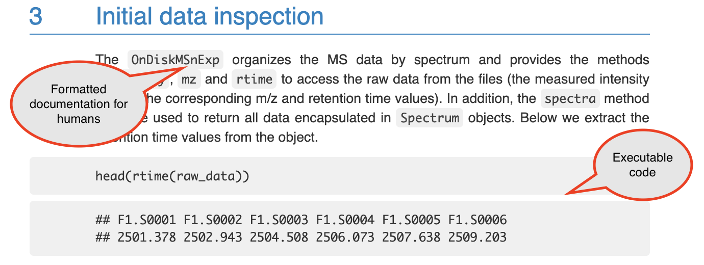
are many tutorials available that are created as knitted documents. Figure
3.1 shows an example from the start of a vignette for the
xcms package in R. This is a package that helps with pre-processing and
analyzing data from LC-MS experiments. You can see that this document includes
text to explain the package and also example code and the output from that code.
Figure 3.1: An example of a knitted document. This shows a section of the online vignette for the xcms package from Bioconductor. The two types of content are highlighted: formatted text for humans to read, and executable computer code.
As a larger example, all the modules in this online book were written as knitted documents. In this module we will describe the characteristics of knitted documents and how the technology behind them works. We will then talk about how you can create them using Rmarkdown. In the next module, we’ll provide an example of doing this for a set of research data from a common laboratory experiment.
The defining characteristic of a knitted document is that it interweaves two
types of content: first, executable code, and, second, documentation that is
formatted in a way that is easy to read. In the figure with the example from the
xcms vignette, we have highlighted the areas that demonstrate these two types
of content (Figure 3.1). Later in this module we will
describe how a knitted document can incorporate these two elements. First,
however, we will explain why you might want to use knitted documents to
document your own research code, especially for pre-processing protocols.
There are several advantages to using knitted documents when writing code to pre-process or analyze research data. These include improvements in terms of reliability, efficiency, transparency, and reproducibility.
First, when you have written your code within a knitted document, this code is checked every time you render the document. In other words, you are checking your code to ensure it operates as you intend throughout the process of writing and editing your document, checking the code each time you render the document to its formatted version. This helps to increase the reliability of the code that you have written. Open-source software evolves over time, and by continuing to check code as you work on protocols and reports with your data, you can ensure that you will quickly identify and adapt to any such changes. Further, you can quickly identify if updates to your research data introduce any issues with the code. Again, by checking the code frequently, you can identify any issues quickly, and this often will allow you to easily pinpoint and fix these issues. By contrast, if you only identify a problem after writing a lot of code, it is often difficult to identify the source of the issue. By including code that is checked each time of document is rendered, you can quickly identify when a change an open source software effects the analysis that you were conducting or the pre-processing and work 2 adapt to any changes quickly.
Second, when you write a document that includes executable code, it allows you to easily rerun the code as you update your research data set, or adopt the code to work with a new data set. If you are not using a knitted document to write pre-processing protocols and research reports, then your workflow is probably to run all your code—either from a script or the command line—and copy the results into a document in a word processing program like Word or Google Docs. If you do that, you must recopy all your results every time you adapt any part of the code or add new data. By contrast, when you use a knitted document, the rendering process executes the code and incorporates the results directly and automatically into a nicely formatted final document. The use of knitted documents therefore can substantially improve the efficiency of pre-processing and analyzing your data and generating the reports that summarize this process.
Third, documents that are created in knitted format are created using plain text. Plain text files can easily be tracked well and clearly using version control tools like git, and associated collaboration tools like GitHub, as discussed in earlier modules. This substantially increases the transparency of the data pre-processing and analysis. It allows you to clearly document changes you or others make in the document, step-by-step. You can document who made the change, and that person can include a message about why they made the change. This full history of changes is recorded and can be searched to explore how the document has evolved and why.
The final advantage of using knitted documents, especially for pre-processing
research data, is that it allows the code to be clearly and thoroughly
documented. This can help increase the reproducibility of the process. In
other words, it can help ensure that another researcher could repeat the same
process, making adaptations as appropriate for their own data set, or ensuring
they arrive at the same results if using the original data. It also ensures that
you can remember exactly what you did, which is especially useful if you plan to
reuse or adopt the code to work with other data sets, as will often be the case
for a pre-processing protocol. If you are not using a knitted document, but are
using code for preprocessing, then as an alternative you may be documenting your
code through comments in a code script. A code script does allow you to include
documentation about the code through these code comments, which are demarcated
from code in the script through a special symbol (# in R). However these code
comments are much less expressive and harder to read than nicely formatted text,
and it is hard to include elements like mathematical equations and literature
citations in code comments. A knitted document allows you to write the
documentation in a format that is clear and attractive for humans to read, while
including code that is clear and easy for a computer to execute.
3.8.4 How knitted documents work
Next, we will describe how knitted documents work. There are seven components of how these documents work. It is helpful to understand these to understand these to begin creating and adapting knitted documents. Knitted documents can be created through a number of programs, and while we will later focus on Rmarkdown, these seven components are in play regardless of the exact system used to create a knitted document, and therefore help in gaining a general understanding of this type of document. We have listed the seven components here and in the following paragraphs will describe each more fully:
- Knitted documents start as plain text;
- A special section at the start of the document (preamble) gives some overall directions about the document;
- Special combinations of characters indicate where the executable code starts;
- Other special combinations show where the regular text starts (and the executable code section ends);
- Formatting for the rest of the document is specified with a markup language;
- You create the final document by rendering the plain text document. This process runs through two software programs; and
- The final document is attractive and read-only—you should never make edits to this output, only to your initial plain text document.
First, a knitted document should be written in plain text. In an earlier module,
we described some of the advantages of using plain text file formats, rather
than proprietary and/or binary file formats, especially in the context of saving
research data (e.g., using csv file formats rather than Excel file formats).
Plain text can also be used to write documentation, including through knitted
documents. Figure 3.2 shows an example of what the plan text might look like for the
start of the xcms tutorial shown in Figure 3.1.
Figure 3.2: An example of a the plain text used to write a knitted document. This shows a section of the plain text used to write the online vignette for the xcms package from Bioconductor. The full plain text file used for the vignette can be viewed on GitHub here.
.](figures/plaintext_vignette_example.png)
There are a few things to keep in mind when writing plain text. First, you should always use a text editor rather than a word processor when you are writing a document in plain text. Text editors can include software programs like Notepad on Microsoft operating systems and TextEdit on Mac operating systems. You can also use a more advanced text editor, like vi/vim or emacs. Rstudio can also serve as a text editor, and if you are doing other work in Rstudio, this is often the most obvious option as a text editor to use to write knitted documents.
You must use a text editor to write plain text for knitted documents for the same reasons that you must use one to write code scripts. Word processors often introduce formatting that is saved through underlying code rather than clearly evident on the document that you see as you type. This hidden formatting can complicate the written text. Conversely, text written in a text editor will not introduce such hard-to-see formatting. Word processing programs also tend to automatically convert some symbols into slightly fancier versions of the symbol. For example, they may change a basic quotation symbol into one with shaping, depending on whether the mark comes at the beginning or end of a quotation. This subtle change in formatting can cause issues in both the code and the formatting specifications that you include in a knitted document.
Further, when are writing plain text, typically you should only use characters from the American Standard Code for Information Interchange, or ASCII. This is a character set from early in computing that includes 128 characters. Such a small character set enforces simplicity: this character set mostly includes what you can see on your keyboard, like the digits 0 to 9, the lowercase and uppercase alphabet, some symbols, including punctuation symbols like the exclamation point and quotation marks, some mathematical symbols like plus, minus, and division, and some control codes, including ones for a new line, a tab, and even ringing a bell. The full set of characters included in ASCII can be found in a number of sources including a very thorough Wikipedia page on this character set (https://en.wikipedia.org/wiki/ASCII).
Because the character set available for plain text files is so small, you will find that it becomes important to leverage the limited characters that are available. One example is white space. White space can be created in ASCII with both the space character and with the new line command. It is an important component that can be used to make plain text files clear for humans to read. As we begin discussing the convention for markdown languages, we will find that white space is often used to help specify formatting as well.
The second component of how knitted documents work is that each knitted document will have a special section at its start called the preamble. This preamble will give some overall directions regarding the document, like its title and authors and the format to which is should be rendered. Knitted documents are created using a markup language to specify formatting for the document, and there are a number of different markup languages including HTML, LaTeX, and Markdown. The specifications for the document’s preamble will depend on the markup language being used.
In Rmarkdown, we will be focusing on Markdown, for which the preamble is specified using something called YAML (short for YAML Ain’t Markup Language). Here is an example of the YAML for a sample pre-processing protocol created using RMarkdown:
  ---
  title: "Preprocessing Protocol for LC-MS Data"
  author: "Jane Doe"
  date: "1/25/2021"
  output: pdf_document
  ---
This YAML preamble specifies information about the document with keys and
values. For example, the title is specified using the YAML key title,
followed by a colon and a space, and then the desired value for that
component of the document, "Preprocessing Protocol for LC-MS Data".
Similarly, the author is specified with the author key and the desired
value for that component, and the date with the date key and associated
component.
Different keys can take different types of values in the YAML
(this is similar to how different parameters in a function can take different values). For example, the keys of author, title, and date all take
a character string with any desired character combination, and the quotation
marks surrounding the values for each of these keys denote those character strings. By contrast, the output key—which specifies the format that
that the knitted document should be rendered to—can only take one of a
few set values, each of which is specified without surrounding
quotation marks (pdf_document in this case, to render the document
as a PDF report).
The rules for which keys can be included in the preamble will depend on the markup language being used. Here, we are showing an example in Markdown, but you can also use other markup languages like LaTeX and HTML, and these will have their own convention for specifying the preamble. Later in this module, when we talk more specifically about Rmarkdown, we will give some resources where you can find more about how to customize the preamble in Rmarkdown specifically. If you are using a different markup language, there are numerous websites, cheatsheets, and other resources you can use to find which keywords are available for the preamble in that markup language, as well as the possible values those keywords can take.
The next characteristic of knitted documents is that they need to clearly demarcate where executable code starts and where regular formatted text starts (in other words, where the executable code section ends). To do this, knitted documents have two special combination of characters, one that can be used in the plain text to indicate where executable code starts and and one to indicate where it ends. For example, Figure 3.3 shows the plain text that could be used in an Rmarkdown document to write some regular text, then some executable code, and then indicate the start of more regular text:
Figure 3.3: An example of how special combinations of characters are used to demarcate code in an RMarkdown file. The color formatting here is applied automatically by RStudio; all the text in this example is written in plain text.
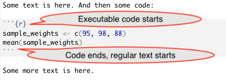
The combination that indicates the start of executable code will vary depending on the markup language being. In Rmarkdown, the following combination indicates the start of executable code:
```{r}
while this combination indicates the end of executable code (in other words the start of regular text):
```
In Figure 3.3 and above, we have shown the most basic
version of the markup character combination used to specify the start of
executable code (```{r}). This character combination can be expanded,
however, to include some specifications for how you want the code in the section
following it to be run, as well as how you want output to be shown. For example,
you could use the following indications to specify that the code should be run,
but the code itself should not be printed in the final document, by specifying
echo = FALSE, as well as that the created figure should be centered on the
page, by specifying fig.align = "center":
```{r echo = FALSE, fig.align = "center"}
There are numerous options that can be used to specify how the code will be run, and later when we talk specifically about Rmarkdown, we will point toward resources that clarify and outline all the possible choices that can be used for these specifications.
You may have noticed that these markers, which indicate the beginning and end of executable code, seem like very odd character combination. There is a good reason for this. By making this character combination unusual, there will be less of a chance that it shows up in regular text. This way there are fewer cases where the writer unintentionally indicate the start of a new section of executable code when trying to write regular text in the knitted document.
The next characteristic of knitted documents is that formatting for the regular
text in the document—that is, everything that is not executable code—is
specified using what is called a markup language. When you were writing in
plain text, you do not have buttons to click on for formatting, for example, to
specify words or phrases that should be in bold or italics, font size, headings,
and so on. Instead you use special characters or character combinations to
specify formatting in the final document. These character combinations are
defined based on the markup language you use. As mentioned earlier, Rmarkdown
uses the Markdown language; other knitted documents can be created using LaTeX
or HTML. As an example of how these special character combinations work, in
Markdown, you place two asterisks around a word or phrase to make it bold. To
write “this” in the final document, in other words, you’ll write
"**this**" in the plain text in the initial document.
You can start to see how this works by looking at the example of the xcms
vignette shown earlier in Figures 3.1 and
3.2. In Figure 3.4, we’ve
recreated these two parts side-by-side, so they’re easier to compare.
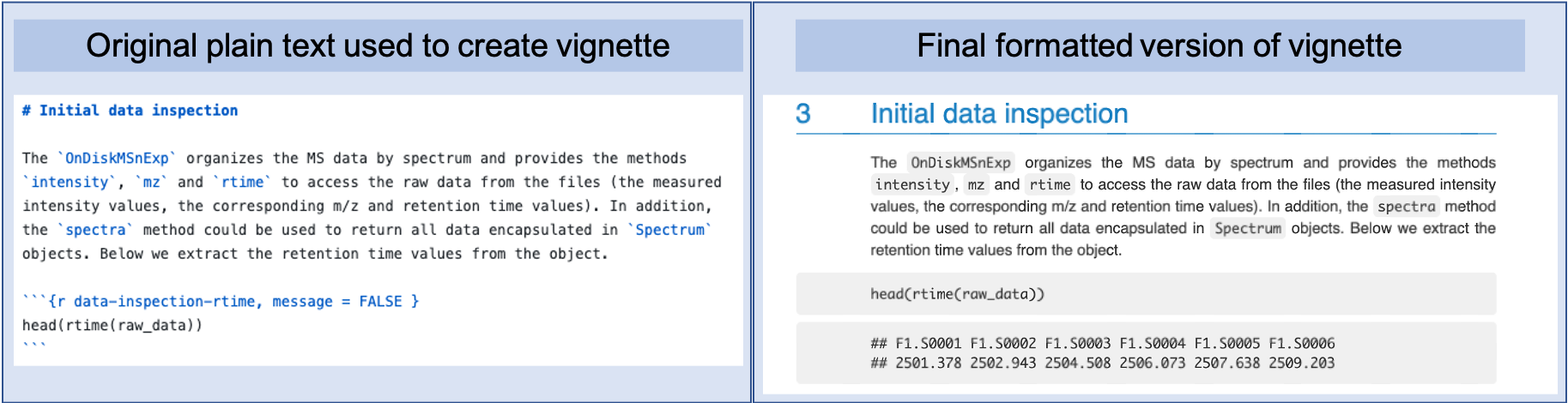
Figure 3.4: The original plain text for a knitted document and the final output, side by side. These examples are from the xcms package vignette, a package available on Bioconductor. The left part of the figure shows the plain text that was written to create the output, which is shown in the left part of the figure. You can see how elements like sections headers and different font styles are indicated in the original plain text through special characters or combinations of charaters, using the Markdown language syntax.
You can look for several formatting elements here. First, the section is headed
“Initial data inspection.” You can that in the original plain text document,
this is marked using a # to start the line with the text for the header. You
can also see that words or phrases that are formatted in a computer-style font
in the final document—to indicate that they are values from computer code,
rather than regular English words—are surrounded by backticks in the plain
text file.
The process of writing your document in this way can feel a little like the old-fashioned style of dictating to a secretary. You can imagine yourself dictating to the computer through the plain text. You have to say not just the words, but also specify in the plain text the formatting that you want at each spot. For example, when you get to a word that you want in italics, you must tell the computer, “Start italics,” then say the word, then “End italics.” You do this using the special formatting characters that are specified by the markup language that you use. Later in this module we will point to resources for discovering all of these formatting specifications for Markdown, the markup language used by RMarkdown.
The final characteristics of knitted documents is that, to create the final document, you will render the plain text document. That is the process that will create an attractive final document. To visualize this, rendering is the process that takes the document from the plain text format, as shown in the left of Figure 3.4, to the final format, shown in the right of that figure.
When you render the document, it will be run through two software programs. The first will look only for sections with executable code, based on the character combination that is used to mark these executable code sections. This first software will execute that code and take any output—including data results, figures, and tables—and insert those at the relevant spot in the document’s file. Next, these output file from this software run will be run through another software program. This second program will look for all the formatting instructions and render the final document in an attractive format. This final output can be in a number of file formats, depending what you specify in the preamble, including a PDF document, an HTML file, or a Word document.
You should consider the final document, regardless of the output format, as read-only. This means that you should never make edits or changes to the final version of the document. Instead you should make any changes to your initial plain text file. This is because the rendering process will overwrite any previous versions of the final document. Therefore any changes that you have made to your final document will be overwritten anytime you re-render from the original plain text document.
3.8.5 Quotes
“It’s very important to keep a project notebook containing detailed information about the chronology of your computational work, steps you’ve taken, information about why you’ve made decisions, and of course all pertinent information to reproduce your work. Some scientists do this in a handwritten notebook, others in Microsoft Word documents. As with README files, bioinformaticians usually like keeping project notebooks in simple plain-text because these can be read, searched, and edited from the command line and across network connections to servers. Plain text is also a future-proof format: plain-text files written in the 1960s are still readable today, whereas files from word processors only 10 years old can be difficult or impossible to open and edit. Additionally, plain text project notebooks can also be put under version control … While plain-text is easy to write in your text editor, it can be inconvenient for collaborators unfamiliar with the command line to read. A lightweight markup language called Markdown is a plain-text format that is easy to read and painlessly incorporated into typed notes, and can also be rendered to HTML or PDF.” (Buffalo 2015)
“Markdown originates from the simple formatting conventions used in plain-text emails. Long before HTML crept into email, emails were embellished with simple markup for emphasis, lists, and blocks of text. Over time, this became a defacto plain-text email formatting scheme. This scheme is very intuitive: underscores or asterisks that flank text indicate emphasis, and lists are simply lines of text beginning with dashes.” (Buffalo 2015)
“Markdown is just plain-text, which means that it’s portable and programs to edit and read it will exist. Anyone who’s written notes or papers in old versions of word processors is likely familiar with the hassle of trying to share or update out-of-date proprietary formats. For these reasons, Markdown makes for a simple and elegant notebook format.” (Buffalo 2015)
“Information, whether data or computer code, should be organized in such a way that there is only one copy of each important unit of information.” (Murrell 2009)
“A typical encounter with Bioconductor (Box 1) starts with a specific scientific need, for example, differential analysis of gene expression from an RNA-seq experiment. The user identifies the appropriate documented workflow, and because the workflow contains functioning code, the user runs a simple command to install the required packages and replicate the analysis locally. From there, she proceeds to adapt the workflow to her particular problem. To this end, additional documentation is available in the form of package vignettes and manual pages.” (Wolfgang Huber et al. 2015)
“Case study: high-throughput sequencing data analysis. Analysis of large-scale RNA or DNA sequencing data often begins with aligning reads to a reference genome, which is followed by interpretation of the alignment patterns. Alignment is handled by a variety of tools, whose output typically is delivered as a BAM file. The Bioconductor packages Rsamtools and GenomicAlignments provide a flexible interface for importing and manipulating the data in a BAM file, for instance for quality assessment, visualization, event detection and summarization. The regions of interest in such analyses are genes, transcripts, enhancers or many other types of sequence intervals that can be identified by their genomic coordinates. Bioconductor supports representation and analysis of genomic intervals with a ‘Ranges’ infrastructure that encompasses data structures, algorithms and utilities including arithmetic functions, set operations and summarization (Fig. 1). It consists of several packages including IRanges, GenomicRanges, GenomicAlignments, GenomicFeatures, VariantAnnotation and rtracklayer. The packages are frequently updated for functionality, performance and usability. The Ranges infrastructure was designed to provide tools that are convenient for end users analyzing data while retaining flexibility to serve as a foundation for the development of more complex and specialized software. We have formalized the data structures to the point that they enable interoperability, but we have also made them adaptable to specific use cases by allowing additional, less formalized userdefined data components such as application-defined annotation. Workflows can differ vastly depending on the specific goals of the investigation, but a common pattern is reduction of the data to a defined set of ranges in terms of quantitative and qualitative summaries of the alignments at each of the sites. Examples include detecting coverage peaks or concentrations in chromatin immunoprecipitation–sequencing, counting the number of cDNA fragments that match each transcript or exon (RNA-seq) and calling DNA sequence variants (DNA-seq). Such summaries can be stored in an instance of the class GenomicRanges.” (Wolfgang Huber et al. 2015)
“Visualization is essential to genomic data analysis. We distinguish among three main scenarios, each having different requirements. The first is rapid interactive data exploration in ‘discovery mode.’ The second is the recording, reporting and discussion of initial results among research collaborators, often done via web pages with interlinked plots and tool-tips providing interactive functionality. Scripts are often provided alongside to document what was done. The third is graphics for scientific publications and presentations that show essential messages in intuitive and attractive forms. The R environment offers powerful support for all these flavors of visualization—using either the various R graphics devices or HTML5-based visualization interfaces that offer more interactivity—and Bioconductor fully exploits these facilities. Visualization in practice often requires that users perform computations on the data, for instance, data transformation and filtering, summarization and dimension reduction, or fitting of a statistical model. The needed expressivity is not always easy to achieve in a point-and-click interface but is readily realized in a high-level programming language. Moreover, many visualizations, such as heat maps or principal component analysis plots, are linked to mathematical and statistical models—for which access to a scientific computing library is needed.” (Wolfgang Huber et al. 2015)
" It can be surprisingly difficult to retrace the computational steps performed in a genomics research project. One of the goals of Bioconductor is to help scientists report their analyses in a way that allows exact recreation by a third party of all computations that transform the input data into the results, including figures, tables and numbers. The project’s contributions comprise an emphasis on literate programming vignettes, the BiocStyle and ReportingTools packages, the assembly of experiment data and annotation packages, and the archiving and availability of all previously released packages. … Full remote reproducibility remains a challenging problem, in particular for computations that require large computing resources or access data through infrastructure that is potentially transient or has restricted access (e.g., the cloud). Nevertheless, many examples of fully reproducible research reports have been produced with Bioconductor." (Wolfgang Huber et al. 2015)
“Using Bioconductor requires a willingness to modify and eventually compose scripts in a high-level computer language, to make informed choices between different algorithms and software packages, and to learn enough R to do the unavoidable data wrangling and troubleshooting. Alternative and complementary tools exist; in particular, users may be ready to trade some loss of flexibility, automation or functionality for simpler interaction with the software, such as by running single-purpose tools or using a point-and-click interface. Workflow and data management systems such as Galaxy and Illumina BaseSpace provide a way to assemble and deploy easy-touse analysis pipelines from components from different languages and frameworks. The IPython notebook provides an attractive interactive workbook environment. Although its origins are with the Python programming language, it now supports many languages, including R. In practice, many users will find a combination of platforms most productive for them.” (Wolfgang Huber et al. 2015)
“A lab manual is perhaps the best way to inform new lab members of the ins and outs of the lab and to keep all members updated on protocols and regulations. What could be included in a lab manual? Anything you do not want to explain over and over, anything that will make the lab more functional and that can make life easier for yourself and lab members.” (LEIPS 2010)
“Most PIs wish the labs were more organized, but it is not a huge priority, that is, until the first student leaves and no one can find a particular cell line in the freezer boxes. Resolutions are made, the crisis passes, and all goes on as before until the next person leaves. Although it is probably inevitable that there will be some confusion when a long-time lab member moves on, an organized lab will not be as affected as an unorganized one.” (LEIPS 2010)
“LaTeX gives you output documents that look great and have consistent cross-references and citations. Much of your output document is created automatically and much is done behind the scenes. This gives you extra time to think about the ideas you want to present and how to communicate those ideas in an effective way.” (Van Dongen 2012)
“LaTeX provides state-of-the-art typesetting” (Van Dongen 2012)
“Many conferences and publishers accept LaTeX. In addition they provide classes and packages that guarantee documents conforming to the required formatting guidelines.” (Van Dongen 2012)
“LaTeX automatically numbers your chapters, sections, figures, and so on.” (Van Dongen 2012)
“LaTeX has excellent bibliography support. It supports consistent citations and an automatically generated bibliography with a consistent look and feel. The style of citations and the organisation of the bibliography is configurable.” (Van Dongen 2012)
“LaTeX is very stable, free, and available on many platforms.” (Van Dongen 2012)
“LaTeX was written by Leslie Lamport as an extension of Donald Knuth’s TeX program. It consists of a Turing-complete procedural markup language and a typesetting processor. The combination of the two lets you control both the visual presentation as well as the content of your documents.” (Van Dongen 2012)
“Roughly speaking LaTeX is built on top of TeX. This adds extra functionality to TeX and makes writing your documents much easier.” (Van Dongen 2012)
“To create a perfect output file and have consistent cross-references and citations, latex also writes information to and reads information from auxiliary files. Auxiliary files contain information about page numbers of chapters, sections, tables, figures, and so on. Some auxiliary files are generated by latex itself (e.g., aux files). Others are generated by external programs such as bibtex, which is a program that generates information for the bibliography. When an auxiliary file changes then LaTeX may be out of sync. You should rerun latex when this happens.” (Van Dongen 2012)
“LaTeX is a markup language and document preparation system. It forces you to focus on the content and not on the presentation. In a LaTeX program you write the content of your document, you use commands to provide markup and automate tasks, and you import libraries.” (Van Dongen 2012)
“The main purpose of [LaTeX] commands is to provide markup. For example, to specify the author of the document you write
\author{<author name>}. The real strength of LaTeX is that it also is a Turing-complete programming language, which lets you define your own commands. These commands let you do real programming and give you ultimate control over the content and the final visual presentation. You can reuse your commands by putting them in a library.” (Van Dongen 2012)
“The paragraph is one of the most important basic building blocks of your document. The paragraph formation rules depend on how latex treats spaces, empty lines, and comments. Roughly, the rules are as follows. In its default model, latex treats a sequence of one or more spaces as a single space. The end of the line is the same as a space. However: An empty line acts as an end-of-paragraph specifier…” (Van Dongen 2012)