Chapter 1 R Preliminaries
The video lectures for this chapter are embedded at relevant places in the text, with links to download a pdf of the associated slides for each video. You can also access a full playlist for the videos for this chapter.
1.1 Objectives
After this chapter, you should:
- Know what free and open source software is and some of its advantages over proprietary software
- Understand the difference between R and RStudio
- Be able to download both R and RStudio to your own computer
- Understand that R has a basic core of code that you initially download, and that this “base R” can be expanded by installing a variety of packages
- Be able to install a package from CRAN to your computer
- Be able to load a package that you have installed to use its functions within an R session
- Be able to access help documentation (vignettes, helpfiles) for a package and its functions
- Be able to submit R expressions at the console prompt to communicate with R
- Understand the structure for calling a function and specifying options for that function
- Know what an R object is and how to assign an R object a name to reference it in later code
- Be able to create vector objects of numeric and character classes
- Be able to explore and extract elements from vector objects
- Be able to create dataframe objects
- Be able to explore and extract elements from dataframe objects
- Be able to describe the difference between running R code from the console versus writing and running R code in an R script
1.2 R and R Studio
Download a pdf of the lecture slides for this video.
1.2.1 What is R?
R in an open-source programming language that evolved from the S language. The S language was developed at Bell Labs in the 1970s, which is the same place (and about the same time) that the C programming language was developed.
R itself was developed in the 1990s–2000s at the University of Auckland. It is open-source software, freely and openly distributed under the GNU General Public License (GPL). The base version of R that you download when you install R on your computer includes the critical code for running R, but you can also install and run “packages” that people all over the world have developed to extend R.
With new developments, R is becoming more and more useful for a variety of programming tasks. However, where it really shines is in working with data and doing statistical analysis. R is currently popular in a number of fields, including:
- Statistics
- Machine learning
- Data analysis
R is an interpreted language. That means that you can communicate with it interactively, from a command line. Other common interpreted languages include Python and Perl.
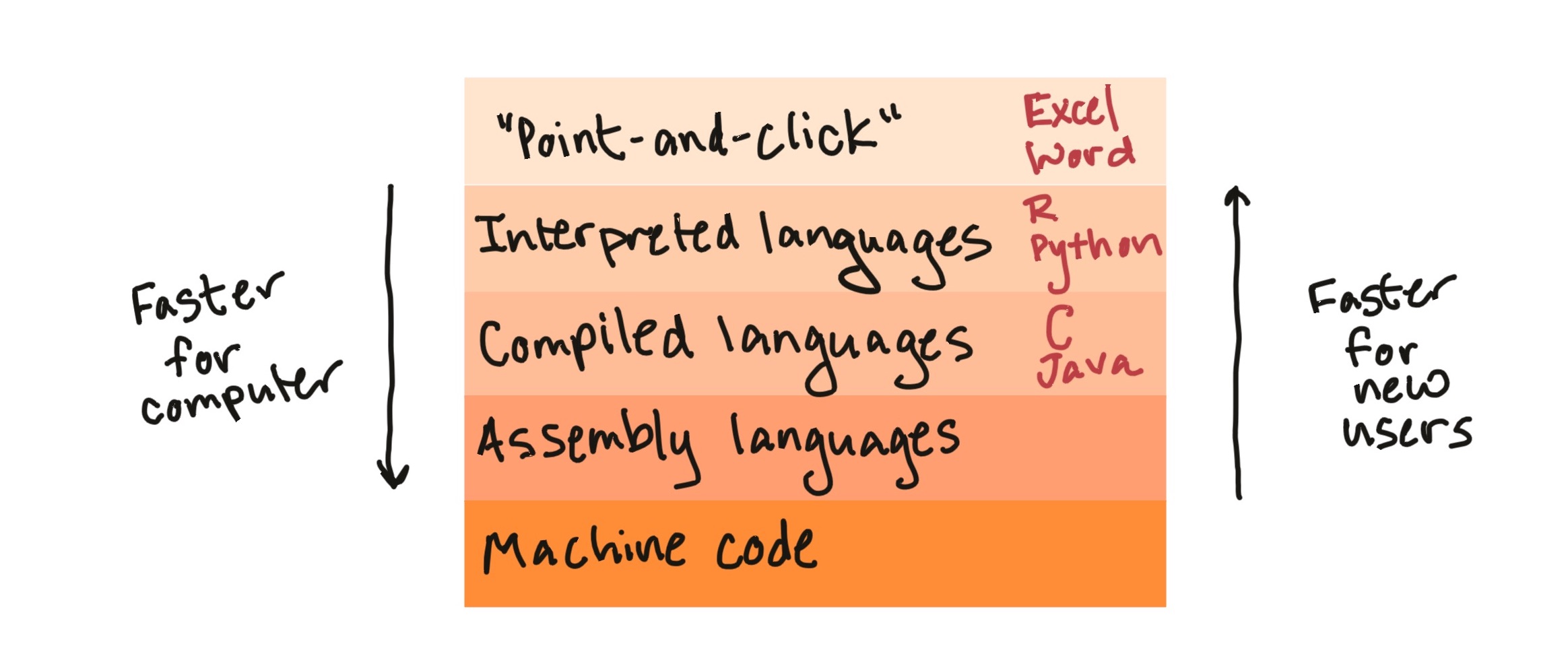
Figure 1.1: Broad types of software programs. R is an interpreted language. ‘Point-and-click’ programs, like Excel and Word, are often easiest for a new user to get started with, but are slower for the computer and are restricted in the functionality they offer. By contrast, compiled languages (like C and Java), assembly languages, and machine code are faster for the computer and allow you to create a wider range of things, but can take longer to code and take longer for a new user to learn to work with.
R has some of the same strengths (quick and easy to code, interfaces well with other languages, easy to work interactively) and weaknesses (slower than compiled languages) as Python. For data-related tasks, R and Python are fairly neck-and-neck (with Julia an up-and-coming option). However, R is still the first choice of statisticians in most fields, so I would argue that R has a an advantage if you want to have access to cutting-edge statistical methods.
“The best thing about R is that it was developed by statisticians. The worst thing about R is that… it was developed by statisticians.” -Bo Cowgill, Google, at the Bay Area R Users Group
1.2.2 Free and open-source software
“Life is too short to run proprietary software.” – Bdale Garbee
R is free and open-source software. Many other popular statistical programming languages, conversely, are proprietary (for example, SAS and SPSS). It’s useful to know what it means for software to be “open-source”, both conceptually and in terms of how you will be able to use and add to R in your own work.
R is free, and it’s tempting to think of open-source software just as “free software”. Things, however, are a little more subtle than that. It helps to consider some different meanings of the word “free”. “Free” can mean:
- Gratis: Free as in beer
- Libre: Free as in speech
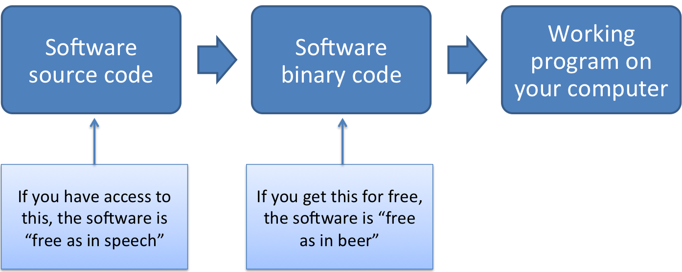
Figure 1.2: An overview of how software can be each type of free (beer and speech). For software programs developed using a compiled programming language, the final product that you open on your computer is run by machine-readable binary code. A developer can give you this code for free (as in beer) without sharing any of the original source code with you. This means you can’t dig in to figure out how the software works and how you can extend it. By contrast, open-source software (free as in speech) is software for which you have access to the human-readable code that was used as in input in creating the software binaries. With open-source code, you can figure out exactly how the program is coded.
Open-source software software is the libre type of free (Figure 1.2). This means that, with software that is open-source, you can:
- Access all of the code that makes up the software
- Change the code as you’d like for your own applications
- Build on the code with your own extensions
- Share the software and its code, as well as your extensions, with others
Often, open-source software is also free, making it “free and open-source software”, or “FOSS”.
Popular open source licenses for R and R packages include the GPL and MIT licenses.
“Making Linux GPL’d was definitely the best thing I ever did.” – Linus Torvalds
In practice, this means that, once you are familiar with the software, you can dig deeply into the code to figure out exactly how it’s performing certain tasks. This can be useful for finding bugs and eliminating bugs, and also can help researchers figure out if there are any limitations in how the code works for their specific research.
It also means that you can build your own software on top of existing R software and its extensions. I explain a bit more about R packages a bit later, but this open-source nature of R (and other languages, including Python) has created a large community of people worldwide who develop and share extensions to R. As a result, you can pull in packages that let you do all kinds of things in R, like visualizing Tweets, cleaning up accelerometer data, analyzing complex surveys, fitting maching learning models, and a wealth of other cool things.
“Despite its name, open-source software is less vulnerable to hacking than the secret, black box systems like those being used in polling places now. That’s because anyone can see how open-source systems operate. Bugs can be spotted and remedied, deterring those who would attempt attacks. This makes them much more secure than closed-source models like Microsoft’s, which only Microsoft employees can get into to fix.” – Woolsey and Fox. To Protect Voting, Use Open-Source Software. New York Times. August 3, 2017.
You can download the latest version of R from
CRAN. Be sure to select the distribution for your
type of computer system. R is updated occasionally; you should plan to
re-install R at least once a year, to make sure you’re working with one of the
newer versions. Check your current R version (one way is by running
sessionInfo() at the R console) to make sure you’re not using an outdated
version of R. Defaults should be fine for everything.
“The R engine … is pretty well uniformly excellent code but you have to take my word for that. Actually, you don’t. The whole engine is open source so, if you wish, you can check every line of it. If people were out to push dodgy software, this is not the way they’d go about it.” - Bill Venables, R-help (January 2004)
“Talk is cheap. Show me the code.” - Linus Torvalds
Download a pdf of the lecture slides for this video.
1.2.3 What is RStudio?
To get the R software, you’ll download R from the R Project for Statistical Computing. This is enough for you to use R on your own computer. However, I would suggest one additional, free piece of software to improve your experience while working with R, RStudio.
RStudio is an integrated development environment (IDE) for R. This basically means that it provides you an interface for running R and coding in R, with a lot of nice extras that will make your life easier.
You download RStudio separately from R—you’ll want to download and install R itself first, and then you can download RStudio. You want the Desktop version with the free license. Defaults should be fine for everything.
RStudio (the company) is a leader in the R community. Currently, the company:
- Develops and freely provides the RStudio IDE
- Provides excellent resources for learning and using R (e.g., cheatsheets, free online books)
- Is producing some of the most-used R packages
- Employs some of the top people in R development
- Is a key member of The R Consortium (others include Microsoft, IBM, and Google)
R has been advancing by leaps in bounds in terms of what it can do and the elegance with which it does it, in large part because of the enormous contributions of people involved with RStudio.
Download a pdf of the lecture slides for this video.
1.3 Communicating with R
Because R is an interpreted language, you can communicate with it interactively. You do this using the following general steps:
- Open an R session
- At the prompt in the console, enter an R expression
- Read R’s “response” (the output)
- Repeat 2 and 3
- Close the R session
1.3.1 R sessions, the console, and the command prompt
An R session is an instance of you using R. To open an R session, double-click on the icon for “RStudio” on you computer. When RStudio opens, you will be in a “fresh” R session, unless you restore a saved session (which I strongly recommend against). This means that, once you open RStudio, you will need to “set up” your session, including loading any packages you need (which we’ll talk about later) and reading in any data (which we’ll also talk about).
In RStudio, there screen is divided into several “panes”. We’ll start with the pane called “Console”. The console lets you “talk” to R. This is where you can “talk” to R by typing an expression at the prompt (the caret symbol, “>”). You press the “Return” key to send this message to R.
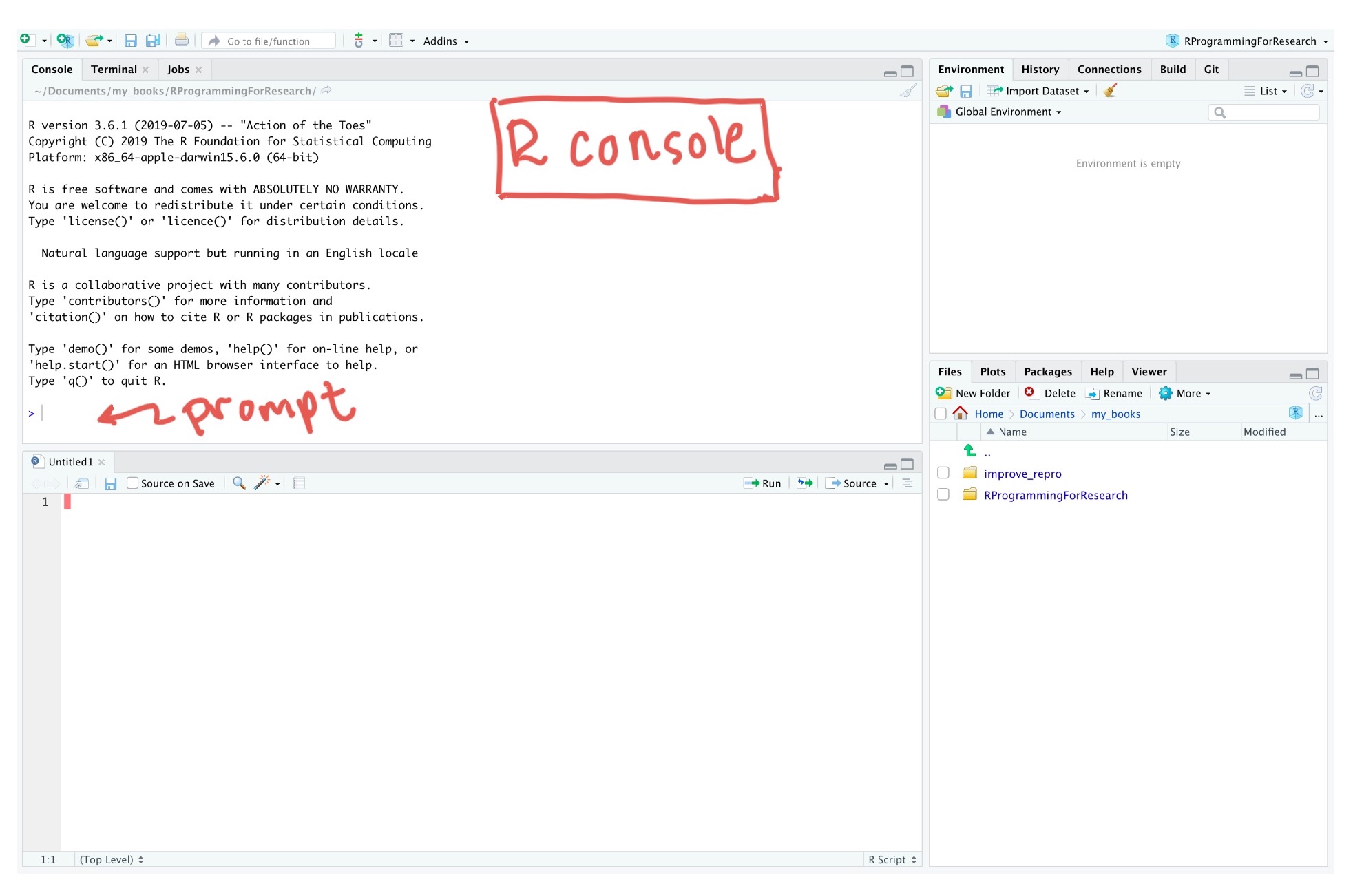
Figure 1.3: Finding the ‘Console’ pane and the command prompt in RStudio.
Once you press “Return”, R will respond in one of three ways:
- R does whatever you asked it to do with the expression and prints the output (if any) of doing that, as well as a new prompt so you can ask it something new
- R doesn’t think you’ve finished asking you something, and instead of giving you a new prompt (“>”) it gives you a “+”. This means that R is still listening, waiting for you to finish asking it something.
- R tries to do what you asked it to, but it can’t. It gives you an error message, as well as a new prompt so you can try again or ask it something new.
1.3.2 R expressions, function calls, and objects
To “talk” with R, you need to know how to give it a complete expression. Most expressions you’ll want to give R will be some combination of two elements:
- Function calls
- Object assignments
We’ll go through both these pieces and also look at how you can combine them together for some expressions.
According to John Chambers, one of the creators of R’s precursor S:
- Everything that exists in R is an object
- Everything that happens in R is a call to a function
Download a pdf of the lecture slides for this video.
1.4 Functions
In general, function calls in R take the following structure:
## Generic code (this won't run)
function_name(formal_argument_1 = named_argument_1,
              formal_argument_2 = named_argument_2,
              [etc.])
Sometimes, we’ll show “generic” code in a code block, that doesn’t actually work if you put it in R, but instead shows the generic structure of an R call. We’ll try to always include a comment with any generic code, so you’ll know not to try to run it in R.
A function call forms a complete R expression, and the output will
be the result of running print or show on the object that is output
by the function call. Here is an example of this structure:
## [1] "Hello world"Figure 1.4 shows an example of the typical elements of a
function call. In this example, we’re calling a function with the name
print. It has one argument, with a formal argument of x, which in
this call we’ve provided the named argument “Hello world”.
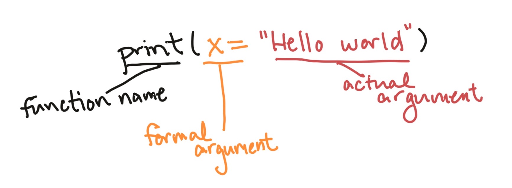
Figure 1.4: Main parts of a function call. This example is calling a function with the name ‘print’. The function call has one argument, with a formal argument of ‘x’, which in this call is provided the named argument ‘Hello world’.
The arguments are how you customize the call to an R function. For example,
you can use change the named argument value to print different messages with the
print function:
## [1] "Hello world"## [1] "Hi Fort Collins"Some functions do not require any arguments. For example, the getRversion function will
print out the version of R you are using.
## [1] '4.4.2'Some functions will accept multiple arguments. For example, the print function allows you
to specify whether the output should include quotation marks, using the quote
formal argument:
## [1] "Hello world"## [1] Hello worldArguments can be required or optional.
For a required argument, if you don’t provide a value for the argument when you
call the function, R will respond with an error. For example, x is a required argument
for the print function, so if you try to call the function without it, you’ll get an
error:
Error in print.default() : argument "x" is
  missing, with no default
For an optional argument on the other hand, R knows a default value for that argument, so if you don’t give it a value for that argument, it will just use the default value for that argument.
For example, for the print function, the quote argument has the default value
TRUE. So if you don’t specify a value for that argument, R will assume it should
use quote = TRUE. That’s why the following two calls give the same result:
## [1] "Hello world"## [1] "Hello world"Often, you’ll want to find out more about a function, including:
- Examples of how to use the function
- Which arguments you can include for the function
- Which arguments are required versus optional
- What the default values are for optional arguments.
You can find out all this information in the function’s helpfile, which
you can access using the function ?. For example, the mean function will let you calculate the mean (average) of a
group of numbers. To find out more about this function, at the console type:
This will open a helpfile in the “Help” pane in RStudio. Figure
1.5 shows some of the key elements of an example helpfile, the
helpfile for the mean function. In particular, the “Usage” section helps you
figure out which arguments are required and which are optional in the
Usage section of the helpfile.
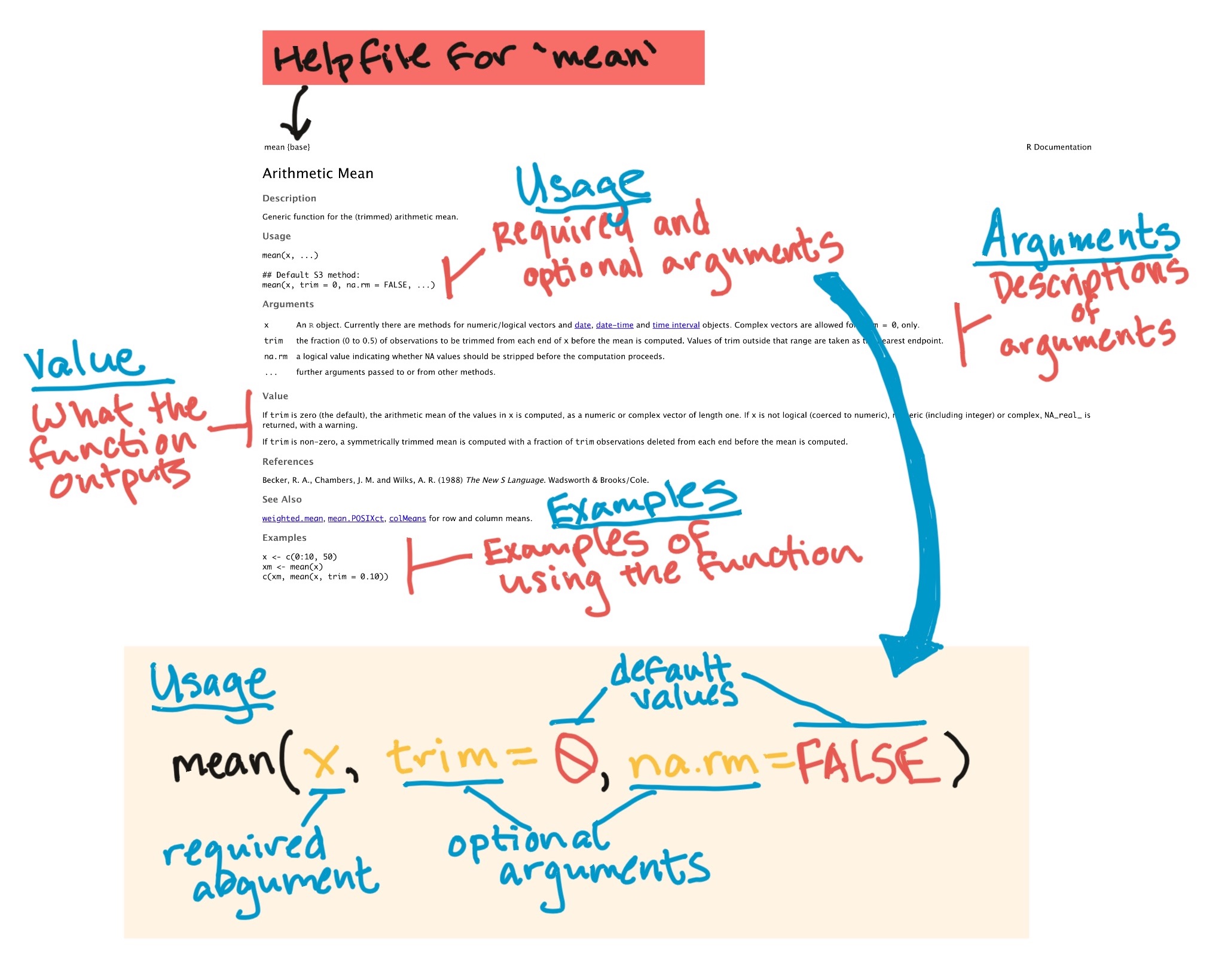
Figure 1.5: Navigating a helpfile. This example shows some key parts of the helpfile for the ‘mean’ function.
There’s one class of functions that looks a bit different from others. These are
the infix operator functions. Instead using parentheses after the function
name, they usually go between two arguments. One common example is the +
operator:
## [1] 5There are operators for several mathematical functions: +, -, *, /.
There are also other operators, including logical operators and assignment
operators, which we’ll cover later.
Download a pdf of the lecture slides for this video.
1.5 Objects and assignment
In R, a variety of different types and structures of data can be saved in what’s called objects. For right now, you can just think of an R object as a discrete container of data in R.
Function calls will produce an object. If you just call a function, as we’ve been doing, then R will respond by printing out that object. However, we’ll often want to use that object some more. For example, we might want to use it as an argument later in our “conversation” with R, when we call another function later. If you want to re-use the results of a function call later, you can assign that object to an object name. This kind of expression is called an assignment expression.
Once you do this, you can use that object name to refer to the object. This means that you don’t need to re-create the object each time you need it—instead you can create it once and then just reference it by name each time you need it after that. For example, you can read in data from an external file as a dataframe object and assign it an object name. Then, when you need that data later, you won’t need to read it in again from the external file.
The gets arrow, <-, is R’s assignment operator. It takes whatever you’ve
created on the right hand side of the <- and saves it as an object with the
name you put on the left hand side of the <- :
For example, if I just type "Hello world", R will print it back to me, but
won’t save it anywhere for me to use later:
## [1] "Hello world"However, if I assign it to an object, I can “refer” to that object in a later expression.
For example, the code below assigns the object "Hello world" the object name message.
Later, I can just refer to this object using the name message, for example in a function
call to the print function:
## [1] "Hello world"When you enter an assignment expression like this at the R console, if everything goes right, then R will “respond” by giving you a new prompt, without any kind of message.
However, there are three ways you can check to make sure that the object was assigned to the object name:
- Enter the object’s name at the prompt and press return. The default if you do this
is for R to “respond” by calling the
printfunction with that object as thexargument. - Call the
lsfunction (which doesn’t require any arguments). This will list all the object names that have been assigned in the current R session. - Look in the “Environment” pane in RStudio. This also lists all the object names that have been assigned in the current R session.
Here’s are examples of these strategies:
- Enter the object’s name at the prompt and press return:
## [1] "Hello world"- Call the
lsfunction:
## [1] "a" "message"- Look in the “Environment” pane in RStudio (see Figure 1.6).
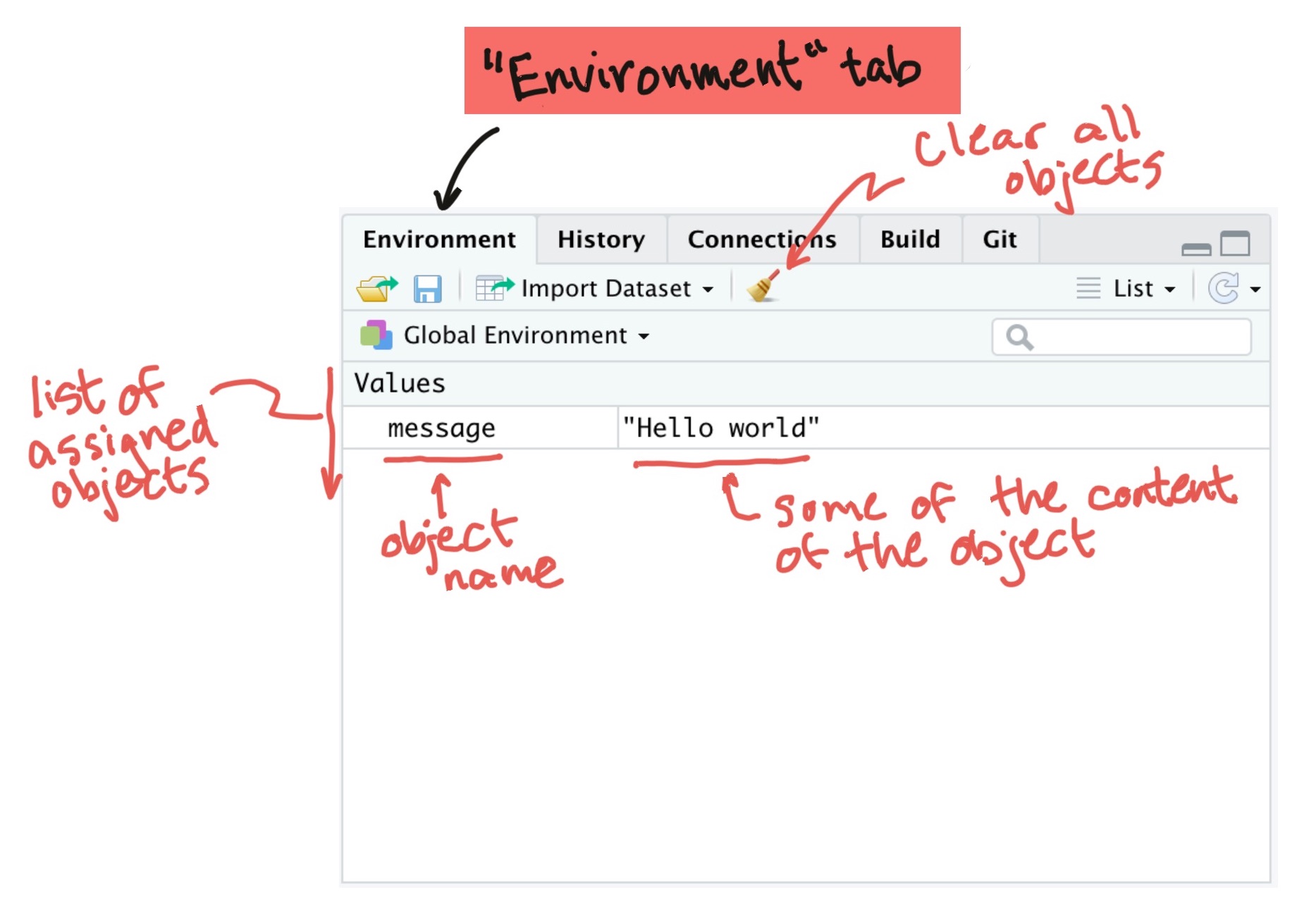
Figure 1.6: ‘Environment’ pane in RStudio. This shows the names and first few values of all objects that have been assigned to object names in the global environment.
You can make assignments in R using either the gets arrow (<-) or =. When
you read other people’s code, you’ll see both. R gurus advise using <- rather
than = when coding in R, and as you move to doing more complex things, some
subtle problems might crop up if you use =. I have heard from someone in the
know that you can tell the age of a programmer by whether he or she uses the
gets arrow or =, with = more common among the young and hip. For this
course, however, I am asking you to code according to Hadley Wickham’s R style
guide, which specifies using the gets arrow
for assignment.
While you will be coding with the gets arrow exclusively in this course, it will be helpful for you to know that the two assignment arrows do pretty much the same thing:
## [1] 1 2 3 4 5 6 7 8 9 10## [1] 1 2 3 4 5 6 7 8 9 10While the gets arrow takes two key strokes instead of one (like the equals sign), you can somewhat get around this limitation by using RStudio’s keyboard shortcut for the gets arrow. This shortcut is Alt + - on Windows and Option + - on Macs. To see a full list of RStudio keyboard shortcuts, go to the “Help” tab in RStudio and select “Keyboard Shortcuts”.
There are some absolute rules for the names you can use for an object name:
- Use only letters, numbers, and underscores
- Don’t start with anything but a letter
If you try to assign an object to a name that doesn’t follow the “hard” rules, you’ll get an error. For example, all of these expressions will give you an error:
In addition to these fixed rules, there are also some guidelines for naming objects that you should adopt now, since they will make your life easier as you advance to writing more complex code in R. The following three guidelines for naming objects are from Hadley Wickham’s R style guide:
- Use lower case for variable names (
message, notMessage) - Use an underscore as a separator (
message_one, notmessageOne) - Avoid using names that are already defined in R (e.g., don’t name an object
mean, because ameanfunction exists)
“Don’t call your matrix ‘matrix’. Would you call your dog ‘dog’? Anyway, it might clash with the function ‘matrix’.” - Barry Rowlingson, R-help (October 2004)
Another good practice is to name objects after nouns (e.g., message) and
later, when you start writing functions, name those after verbs (e.g.,
print_message). You’ll want your object names to be short enough that they
don’t take forever to type as you’re coding, but not so short that you can’t
remember what they stand for.
Sometimes, you’ll want to create an object that you won’t want to keep for very long. For example, you might want to create a small object to test some code, but you plan to not need the object again once you’ve done that. You may want to come up with some short, generic object names that you use for these kinds of objects, so that you’ll know that you can delete them without problems when you want to clean up your R session.
There are all kinds of traditions for these placeholder variable
names in computer science. foo and bar are two
popular choices, as are, evidently, xyzzy,
spam, ham, and norf. There are
different placeholder names in different languages: for example,
toto, truc, and azerty (French);
and pippo, pluto, paperino
(Disney character names; Italian). See the Wikipedia page on metasyntactic
variables to find out more.
Download a pdf of the lecture slides for this video.
1.6 More on communicating with R
What if you want to “compose” a call from more than one function call? One way to do it is to assign the output from the first function call to a name and then use that name for the next call. For example:
## [1] "Hello world"If you give two objects the same name, the most recent definition will be used (i.e., objects can be overwritten by assigning new content to the same object name). For example:
## [1] 1 2 3 4 5 6 7 8 9 10## [1] "A" "B" "C"## [1] "A" "B" "C"To create an R expression you can “nest” one function call inside another function call. For example:
## [1] "Hello world"Just like with math, the order that the functions are evaluated moves from the inner set of parentheses to the outer one (Figure 1.7). There’s one more way we’ll look at later called “piping”.
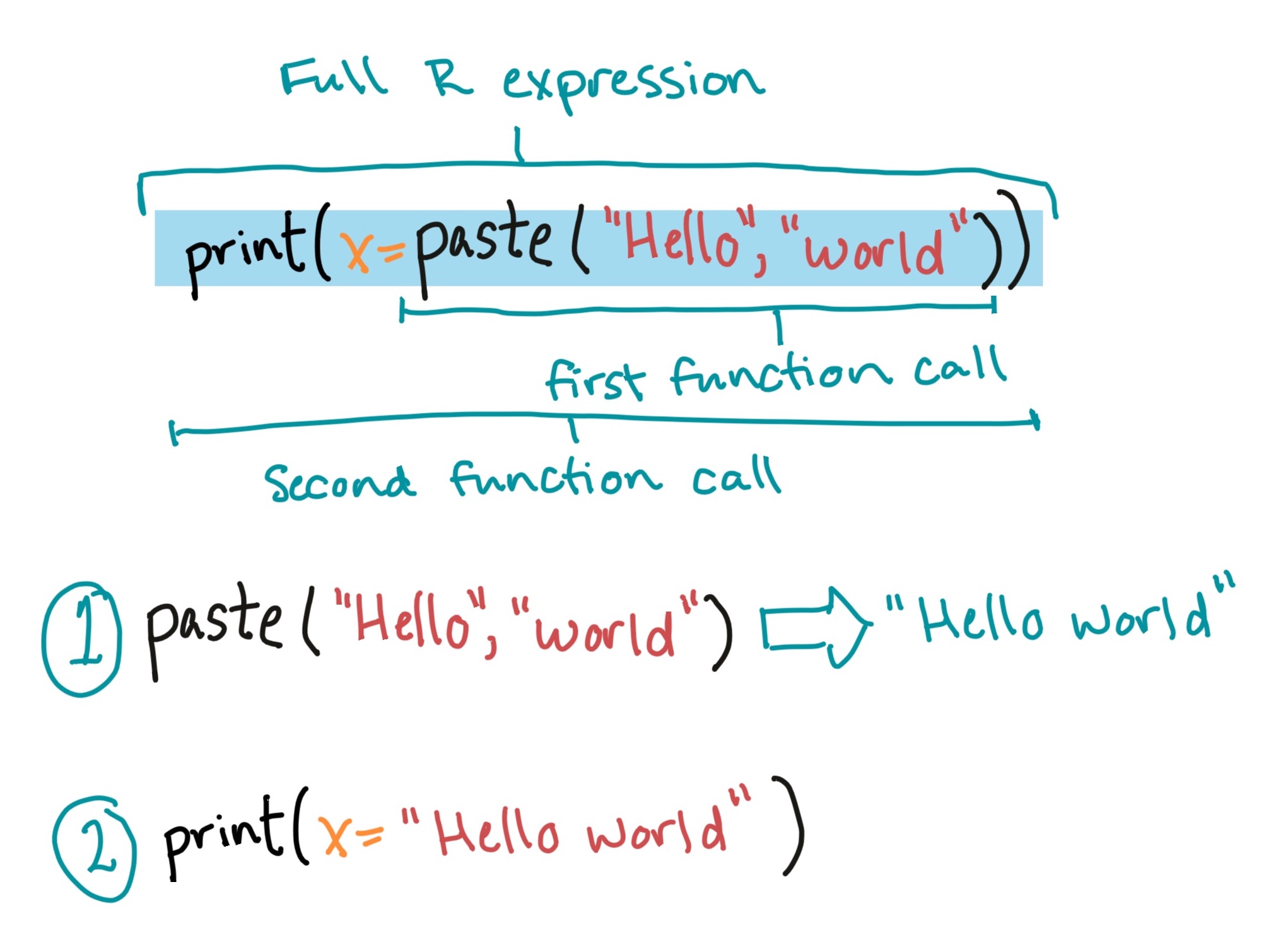
Figure 1.7: ‘Environment’ pane in RStudio. This shows the names and first few values of all objects that have been assigned to object names in the global environment.
1.7 R scripts
This is a good point in learning R for you to start putting your code in R scripts, rather than entering commands at the console.
An R script is a plain text file where you can save a series of R commands. You can save the script and open it up later to see (or re-do) what you did earlier, just like you could with something like a Word document when you’re writing a paper. To open a new R script in RStudio, go to the menu bar and select “File” -> “New File” -> “R Script”. Alternatively, you can use the keyboard shortcut Command-Shift-N. Figure 1.8 gives an example of an R script file opened in RStudio and points out some interesting elements.
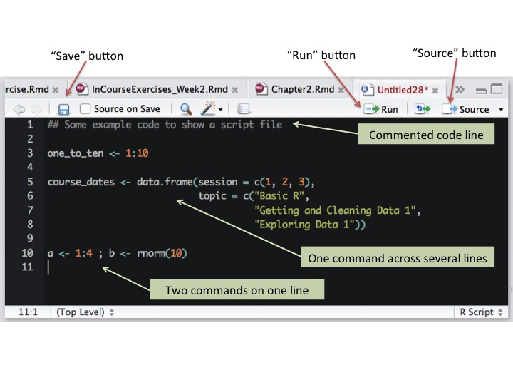
Figure 1.8: Example of an R script in RStudio.
To save a script you’re working on, you can click on the “Save” button (which looks like a floppy disk) at the top of your R script window in RStudio or use the keyboard shortcut Command-S. You should save R scripts using a “.R” file extension.
Within the R script, you’ll usually want to type your code so there’s one
command per line. If your command runs long, you can write a single call over
multiple lines. It’s unusual to put more than one command on a single line of a
script file, but you can if you separate the commands with semicolons (;).
These rules all correspond to how you can enter commands at the console.
Running R code from a script file is very easy in RStudio. You can use either the “Run” button or Command-Return, and any code that is selected (i.e., that you’ve highlighted with your cursor) will run at the console. You can use this functionality to run a single line of code, multiple lines of code, or even just part of a specific line of code. If no code is highlighted, then R will instead run all the code on the line with the cursor and then move the cursor down to the next line in the script.
You can also run all of the code in a script. To do this, use the “Source”
button at the top of the script window. You can also run the entire script
either from the console or from within another script by using the source()
function, with the filename of the script you want to run as the argument. For
example, to run all of the code in a file named “MyFile.R” that is saved in your
current working directory, run:
You can add comments into an R script to let others know (and remind yourself)
what you’re doing and why. To do this, use R’s comment character, #. Any line
on a script line that starts with # will not be read by R. You can also take
advantage of commenting to comment out certain parts of code that you don’t want
to run at the moment.
While it’s generally best to write your R code in a script and run it from there
rather than entering it interactively at the R console, there are some
exceptions. A main example is when you’re initially checking out a dataset, to
make sure you’ve read it in correctly. It often makes more sense to run commands
for this task, like str(), head(), tail(), and summary(), at the
console. These are all examples of commands where you’re trying to look at
something about your data right now, rather than code that builds toward
your analysis, or helps you read in or clean up your data.
1.7.1 Commenting code
Sometimes, you’ll want to include notes in your code. You can do this in all
programming languages by using a comment character to start the line with your
comment. In R, the comment character is the hash symbol, #. R will skip any
line that starts with # in a script. For example, if you run the following
code:
## [1] "But print this"R will only print the second, uncommented line.
You can also use a comment in the middle of a line, to add a note on what you’re doing in that line of the code. R will skip any part of the code from the hash symbol on. For example:
## [1] "Print this"There’s typically no reason to use code comments when running commands at the R console. However, it’s very important to get in the practice of including meaningful comments in R scripts. This helps you remember what you did when you revisit your code later.
“You know you’re brilliant, but maybe you’d like to understand what you did 2 weeks from now.” – Linus Torvalds
Download a pdf of the lecture slides for this video.
1.8 The “package” system
1.8.1 R packages
“Any doubts about R’s big-league status should be put to rest, now that we have a Sudoku Puzzle Solver. Take that, SAS!” - David Brahm (announcing the sudoku package), R-packages (January 2006)
Your original download of R is only a starting point. You can expand functionality of R with what are called packages, or extensions with new code and functionality that add to the basic “base R” environment. To me, this is a bit like the toy train set that my son was obsessed with for a while. You first buy a very basic set that looks something like Figure 1.9.
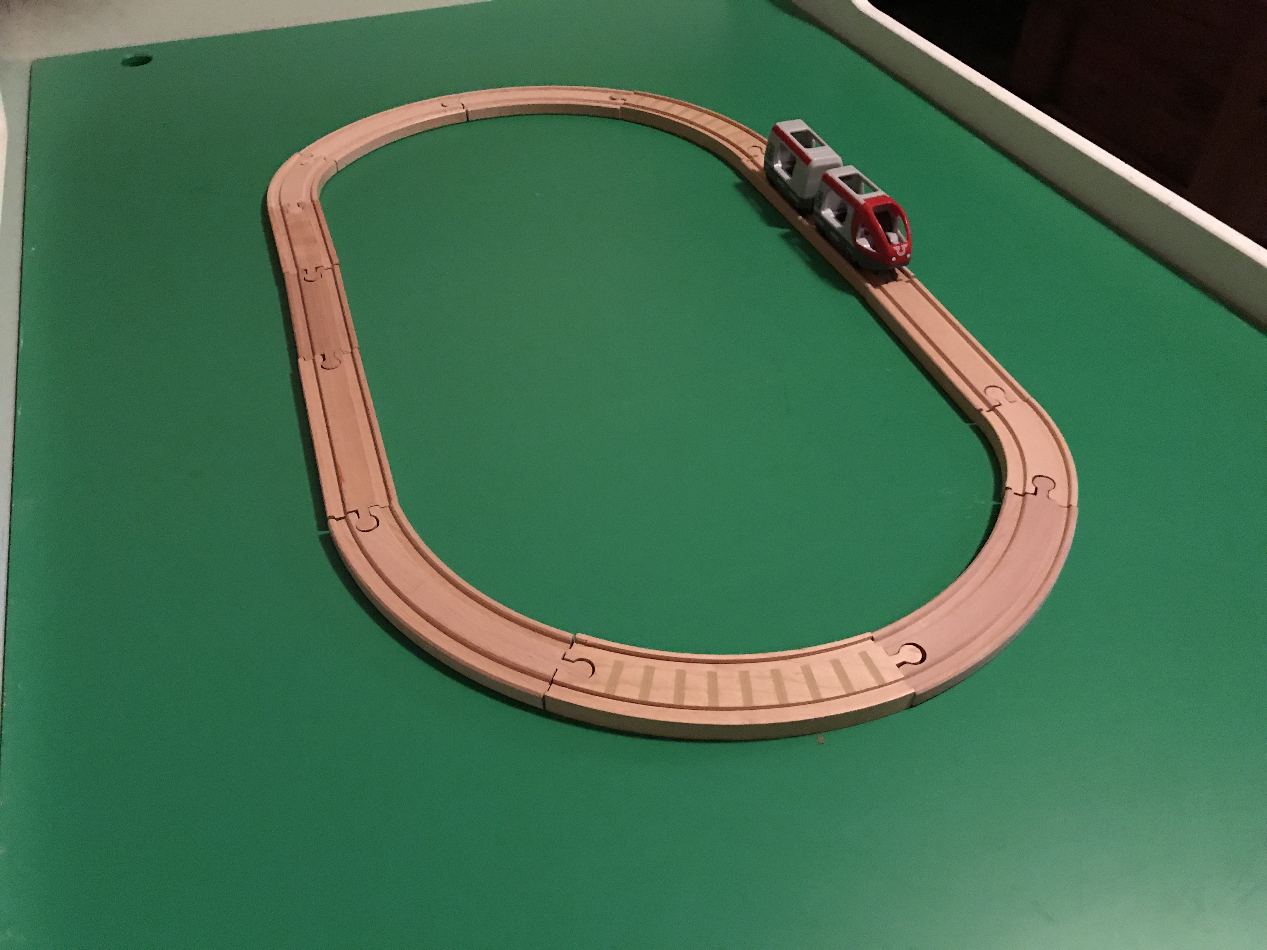
Figure 1.9: The toy version of base R.
To take full advantage of R, you’ll want to add on packages. In the case of the train set, at this point, a doting grandparent adds on extensively through birthday presents, so you end up with something that looks like Figure 1.10.
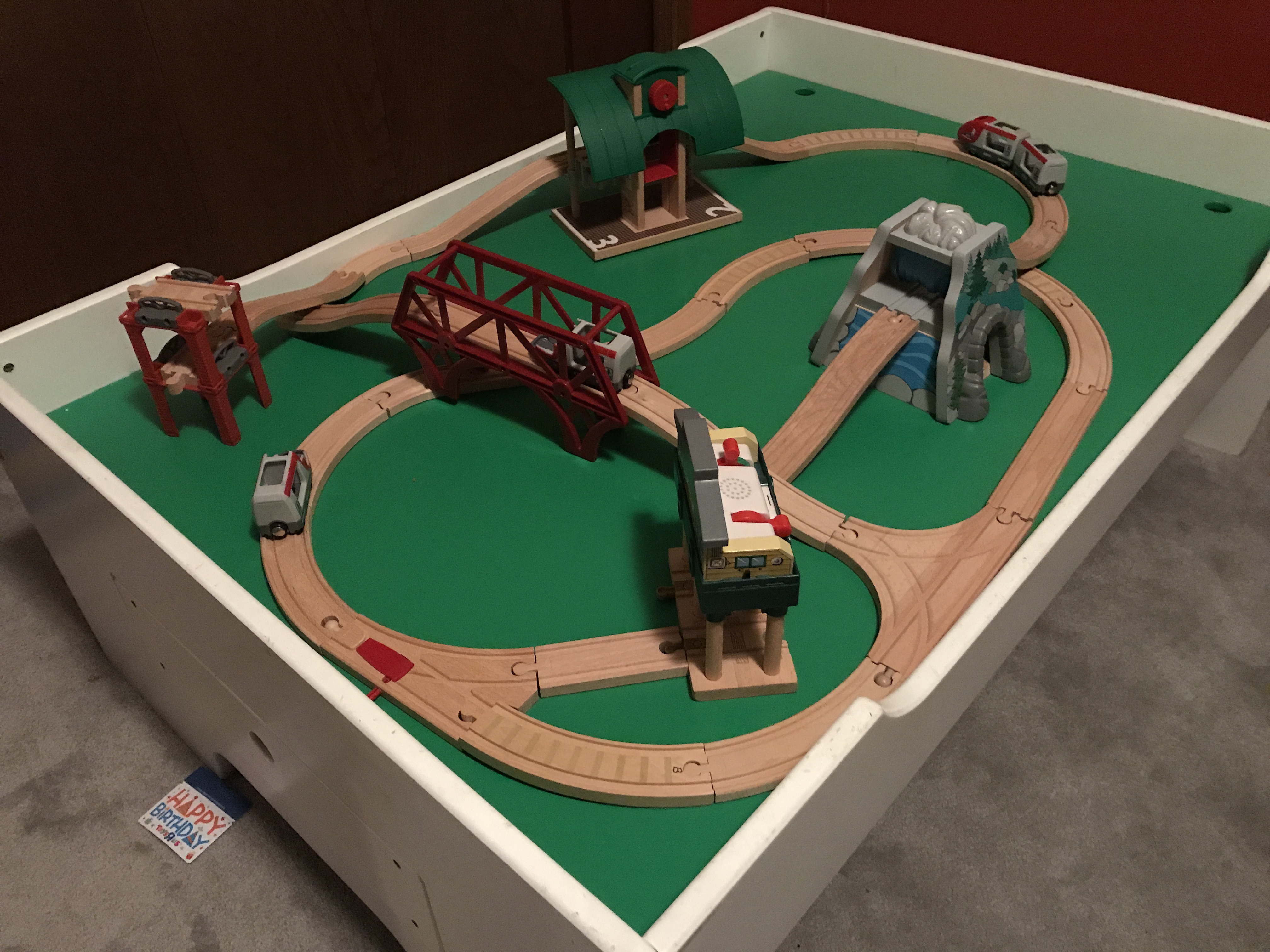
Figure 1.10: The toy version of what your R set-up will look like once you find cool packages to use for your research.
Each package is basically a bundle of extra R functions. They may also include help documentation, datasets, and some other objects, but typically the heart of an R package is the new functions it provides.
You can get these “add-on” packages in a number of ways. The main source for installing packages for R remains the Comprehensive R Archive Network, or CRAN. However, GitHub is growing in popularity, especially for packages that are still in development. You can also create and share packages among your collaborators or co-workers, without ever posting them publicly. In the “Advanced” section of this course, you will learn some about writing your own R package.
1.8.2 Installing from CRAN
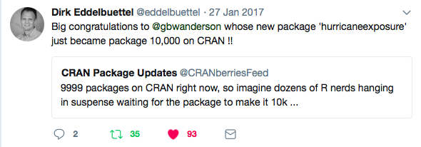
Figure 1.11: Celebrating CRAN’s 10,000th package.
The most popular place from which to get packages is currently CRAN, which has
over 10,000 R packages available (Figure 1.11). You can install
packages from CRAN using R code, with the install.packages function. For
example, telephone keypads include letters for each number (Figure
1.12), which allow companies to have “named” phone numbers
that are easier for people to remember, like 1-800-GO-FEDEX and 1-800-FLOWERS.
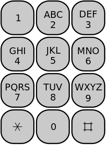
Figure 1.12: Telephone keypad with letters corresponding to each number.
The phonenumber package is a cool little package that will convert between
numbers and letters based on the telephone keypad. Since this package is on
CRAN, you can install the package to your computer using the install.packages
function:
This downloads the package from CRAN and saves it in a special location on your
computer where R can load it when you’re ready to use it. Once you’ve installed
a package to your computer this way, you don’t need to re-run this
install.packages for the package ever again (unless the package maintainer
posts an updated version).
Just like R itself, packages often evolve and are updated by their maintainers. You should update your packages as new versions come out. Typically, you have to reinstall packages when you update your version of R, so this is a good chance to get the most up-to-date version of the packages you use.
1.8.3 Loading an installed package
Once you have installed a package, it will be saved to your computer. However, you won’t be able to access its functions within an R session until you load it in that R session. Loading a package essentially makes all of the package’s functions available to you.
You can load a package in an R session using the
library function, with the package name inside the parentheses.
Figure 1.13 provides a conceptual picture of the different steps of installing and loading a package.
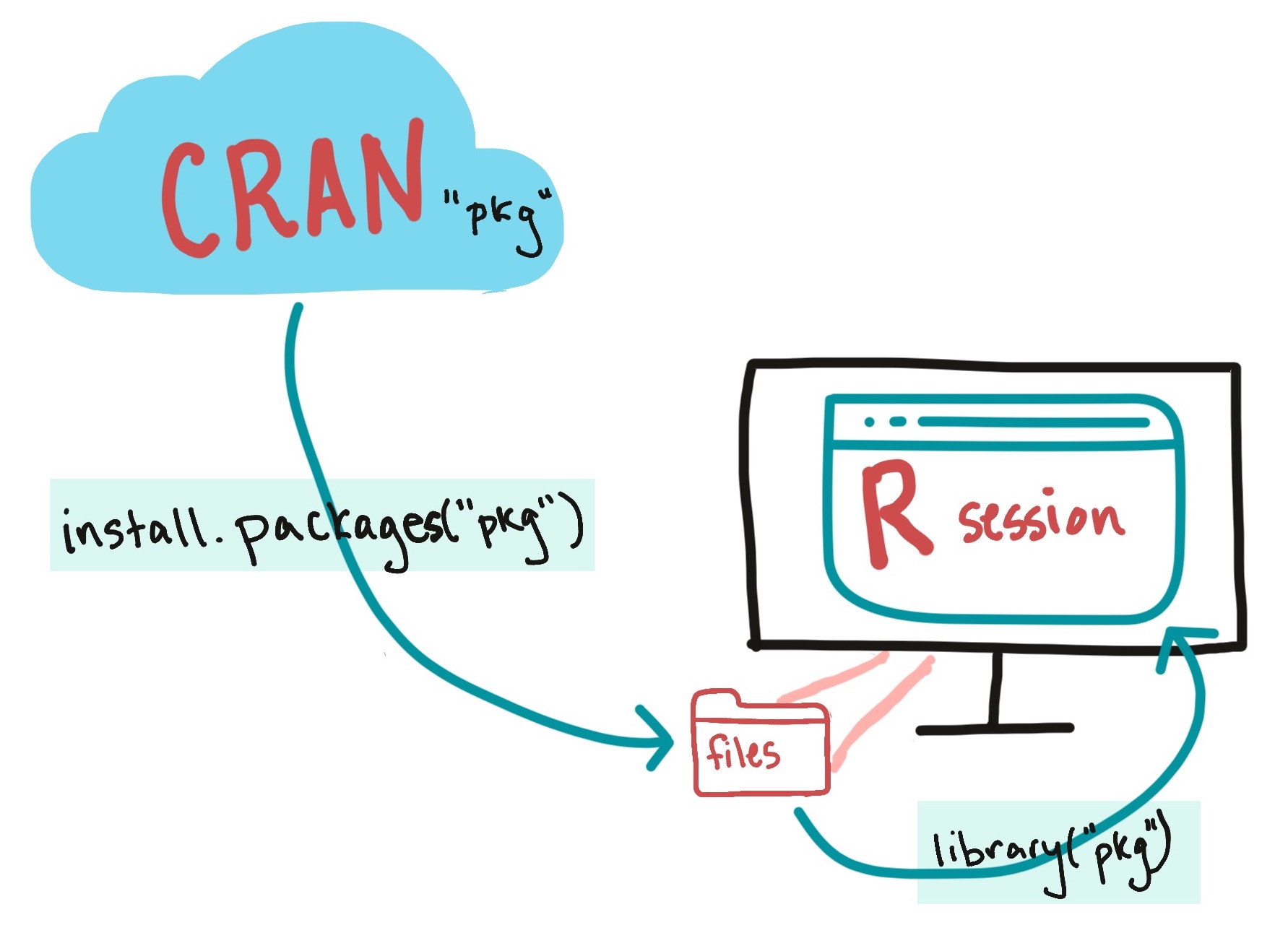
Figure 1.13: Install a package (with ‘install.packages’) to get it onto your computer. Load it (with ‘library’) to get it into your R session.
Once a package is loaded, you can use all its exported (i.e., public) functions
by calling them directly. For example, the phonenumber has a function called
letterToNumber that converts a character string to a number. If you have not
loaded the phonenumber package in your current R session and try to use this
function, you will get an error. However, once you’ve loaded phonenumber using
the library function, you can use this function in your R session:
## [1] "4633339"R vectors can have several different classes. One common class is the character class, which is the class of the character string we’re using here (“GoFedEx”). You’ll always put character strings in quotation marks. Another key class is numeric (numbers). Later in the course, we’ll introduce other classes that vectors can have, including factors and dates. For the simplest vector classes, these classes are determined by the type of data that the vector stores.
When you open RStudio, unless you reload the history of a previous R session (which I typically strongly do not recommend), you will start your work in a “fresh” R session. This means that, once you open RStudio, you will need to run the code to load any packages, define any objects, and read in any data that you will need for analysis in that session.
If you are using a package in academic research, you should cite it, especially
if it implements an algorithm or method that is not standard. You can use the
citation function to get the information you need about how to cite a package:
## To cite package 'phonenumber' in publications use:
##
##   Myles S (2021). _phonenumber: Convert Letters to Numbers and Back as
##   on a Telephone Keypad_. R package version 0.2.3,
##   <https://CRAN.R-project.org/package=phonenumber>.
##
## A BibTeX entry for LaTeX users is
##
##   @Manual{,
##     title = {phonenumber: Convert Letters to Numbers and Back as on a Telephone Keypad},
##     author = {Steve Myles},
##     year = {2021},
##     note = {R package version 0.2.3},
##     url = {https://CRAN.R-project.org/package=phonenumber},
##   }
We’ve talked here about loading packages using the
library function to access their functions. However, this
is not the only way to access the package’s functions. The syntax
[package name]::[function name] (e.g.,
phonenumber::letterToNumber(fedex)) will allow you to use a
function from a package you have installed on your computer, even if its
package has not been loaded in the current R session. Typically, this
syntax is not used much in data analysis scripts, in part because it
makes the code much longer. However, you will occassionally see it used
to distinguish between two functions from different packages that have
the same name, as this format makes the desired function unambiguous.
One example where this syntax often is needed is when both
plyr and dplyr packages are loaded in an R
session, since these share functions with the same name.
Packages typically include some documentation to help users. These include:
- Package vignettes: Longer, tutorial-style documents that walk the user through the basics of how to use the package and often give some helpful example cases of the package in use.
- Function helpfiles: Files for each external function (i.e., the package maintainer wants it to be used by others) within the package, following an established structure. These include information about what inputs are required and optional for the function, what output will be created, and what options can be selected by the user. In many cases, these also include examples of using the function.
To determine which vignettes are available for a package, you can use the
vignette function, with the package’s name specified for the package option:
From the output of this, you can call any of the package’s vignettes directly.
For example, the previous call tells you that this package only has one
vignette, and that vignette has the same name as the package (“phonenumber”).
Once you know the name of the vignette you would like to open, you can also use
vignette to open it:
To access the helpfile for any function within a package you’ve loaded, you can
use ? followed by the function’s name:
Download a pdf of the lecture slides for this video.
1.9 R’s most basic object types
An R object stores some type of data that you want to use later in your R code,
without fully recreating it. The content of R objects can vary from very simple
(the "GoFedEx" string in the example code above) to very complex objects with
lots of elements (for example, a machine learning model).
Objects can be structured in different ways, in terms of how they “hold” data. These difference structures are called object classes. One class of objects can be a subtype of a more general object class.
There are a variety of different object types in R, shaped to fit different types of objects ranging from the simple to complex. In this section, we’ll start by describing two object types that you will use most often in basic data analysis, vectors (1-dimensional objects) and dataframes (2-dimensional objects).
For these two object classes (vectors and dataframes), we’ll look at:
- How that class is structured
- How to make a new object with that class
- How to extract values from objects with that class
In later classes, we’ll spend a lot of time learning how to do other things with objects from these two classes, plus learn some other classes.
1.9.1 Vectors
To get an initial grasp of the vector object type in R, think of it as a 1-dimensional object, or a string of values. Figure 1.14 provides an example of the structure for a very simple vector, one that holds the names of the three main characters in the Harry Potter book series.
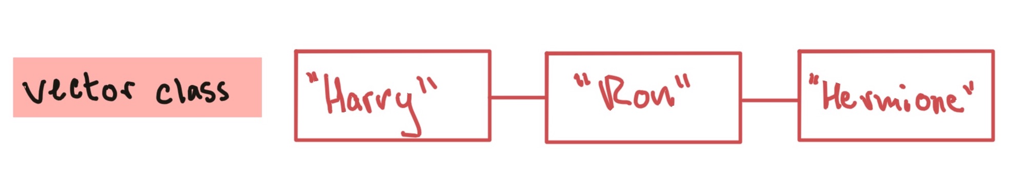
Figure 1.14: An example of the structure of an R object with the vector class. This object class contains data as a string of values, all with the same data type.
All values in a vector must be of the same data type (i.e., all numbers, all characters, all dates). If you try to create a vector with elements from different types (like “FedEx”, which is a character, and 3, a number), R will coerce all of the elements to the most generic type of any of the elements (i.e., “FedEx” and “3” will both become characters, since “3” can be changed to a character, but “FedEx” can’t be changed to a number). Figure 1.15 gives some examples of different classes of vectors.
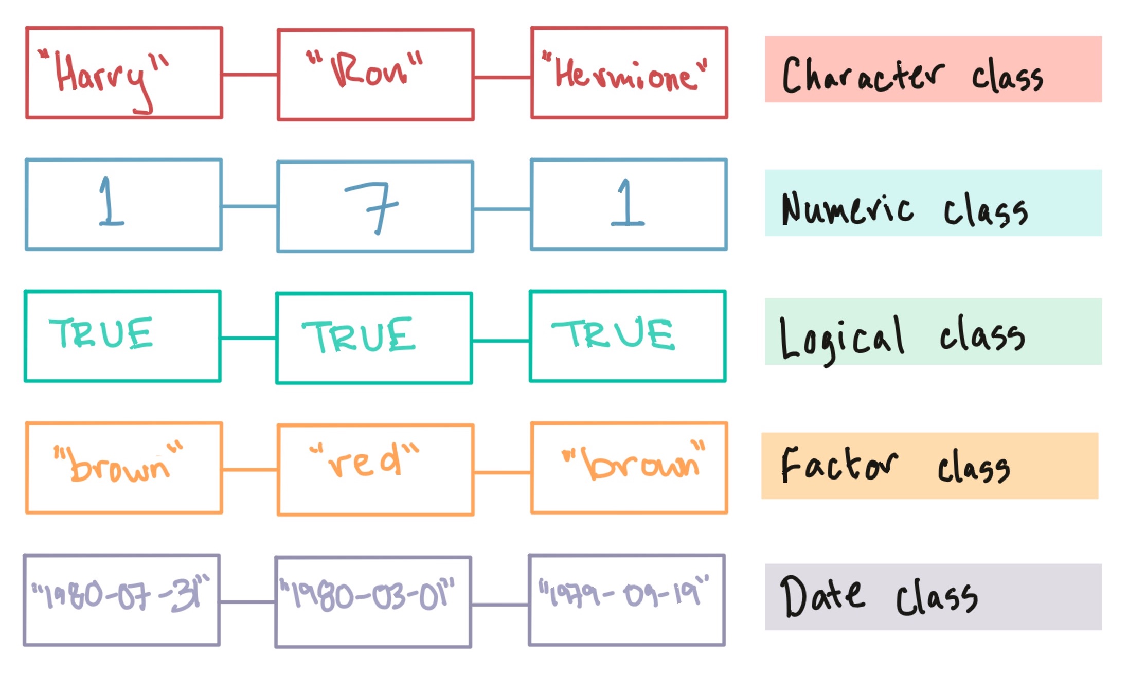
Figure 1.15: Examples of vectors of different classes. All the values in a vector must be of the same type (e.g., all numbers, all characters). There are different classes of vectors depending on the type of data they store.
To create a vector from different elements, you’ll use the concatenation
function, c to join them together, with commas between the elements. For
example, to create the vector shown in Figure 1.14, you
can run:
## [1] "Harry" "Ron" "Hermione"If you want to use that object later, you can assign it an object name in the expression:
## [1] "Harry" "Ron" "Hermione"This assignment expression, for assigning a vector an object name, follows the structure we covered earlier for function calls and assignment expressions (Figure 1.16).
Figure 1.16: Elements of the assignment expression for creating a vector and assigning it an object name.
If you create a numeric vector, you should not put the values in quotation marks:
If you mix classes when you create the vector, R will coerce all the elements to most generic of the elements’ classes:
## [1] "1" "3" "five"Notice that the two integers, 1 and 3, are now in quotation marks, once they
are put in a vector with a value with the character data type. You can use the
class function to determine the class of an object:
## [1] "character"A vector’s length is the number of elements in the vector. You can use the
length function to determine a vector’s length:
## [1] 3Once you create an object, you will often want to reference the whole object in
future code. However, there will be some times when you’ll want to reference
just certain elements of the object (for example, the first three values). You
can pull out certain values from a vector by using indexing with square brackets
([...]) to identify the locations of the element you want to extract. For
example, to extract the second element of the main_characters vector, you can
run:
## [1] "Ron"You can use this same method to extract more than one value. You just need to
create a numeric vector with the position of each element you want to extract
and pass that in the square brackets. For example, to extract the first and
third elements of the main_characters vect, you can run:
## [1] "Harry" "Hermione"The : operator can be very helpful with extracting values from a vector.
This operator creates a sequence of values from the value before the : to the
value after :, going by units of 1. For example, if you want to create a list
of the numbers between 1 and 10, you can run:
## [1] 1 2 3 4 5 6 7 8 9 10If you want to extract the first two values from the main_characters vector, you
can use the : operator:
## [1] "Harry" "Ron"You can also use logic to pull out some values of a vector. For example, you
might only want to pull out even values from the fibonacci vector. We’ll cover
using logical expressions to index vectors later in the book.
One thing that people often find confusing when they start using R is
knowing when to use and not use quotation marks. The general rule is
that you use quotation marks when you want to refer to a character
string literally, but no quotation marks when you want to refer to the
value in a previously-defined object. For example, if you saved the
string “Anderson” as the object my_name
(my_name <- “Anderson”), then in later code, if you type
my_name (no quotation marks), you’ll get
“Anderson”, while if you type out “my_name”
(with quotation marks), you’ll get “my_name” (what you
typed, literally).
One thing that makes this rule confusing is that there are a few
cases in R where you really should (by this rule) use quotation marks,
but the function is coded to let you be lazy and get away without them.
One example is the library function. In the code earlier in
this section to load the “phonenumber” package, you want to literally
load the package “phonenumber”, rather than load whatever character
string is saved in the object named phonenumber. However,
library is one of the functions where you can be lazy and
skip the quotation marks, and it will still load “phonenumber” for you.
Therefore, if you want, this function also works if you call
library(package = phonenumber) (without the quotation
marks) instead of how we actually called it
(library(package = phonenumber)).
Download a pdf of the lecture slides for this video.
1.9.2 Dataframes
A dataframe is a 2-dimensional object, and is made of one or more vectors of the same length stuck together side-by-side. It is the closest R has to an Excel spreadsheet-type structure. Figure 1.17 gives a conceptual example of a dataframe created from several of the vector examples in Figure ??.
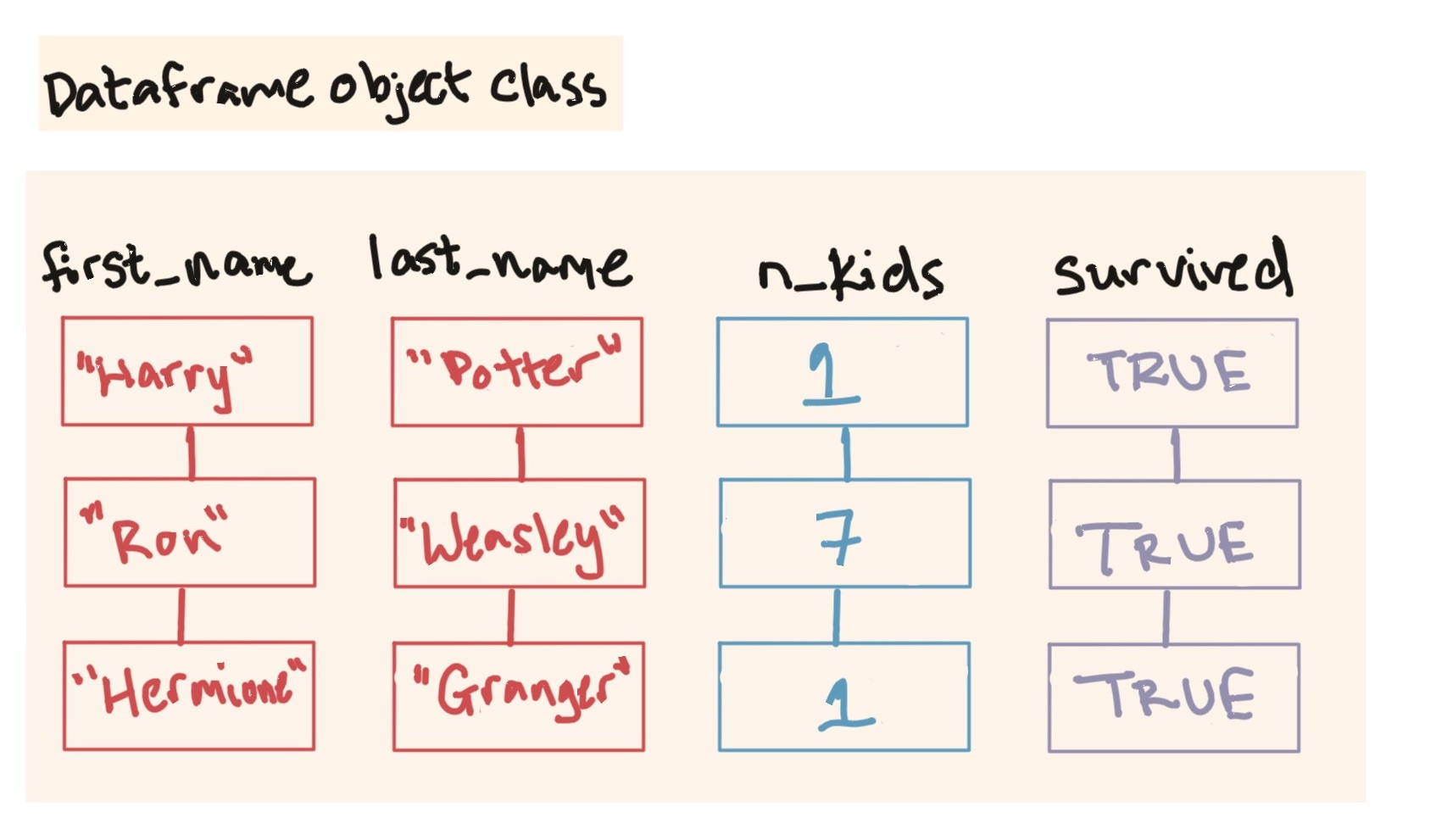
Figure 1.17: An example dataframe, created from several vectors of the same length and with observations aligned across vector positions (for example, the first value in each vector provides a value for Harry, the second for Ron).
Here’s how the dataframe in Figure 1.17 will look in R:
## # A tibble: 3 × 4
##   first_name last_name n_kids survived
##   <chr>      <chr>      <dbl> <lgl>
## 1 Harry      Potter         1 TRUE
## 2 Ron        Weasley        7 TRUE
## 3 Hermione   Granger        1 TRUE
This dataframe is arranged in rows and columns, with column names for each
column (Figure 1.18). Note that each row of this
dataframe gives a different observation (in this case, our unit of observation
is a Harry Potter character). Each column gives a different type of information
(first name, last name, birth year, and whether they’re still alive) for each of
the observations (Beatles). Notice that the number of elements in each of the
columns must be the same in this dataframe, but that the different columns can
have different classes of data (e.g., character vectors for first_name and
last_name, logical value of TRUE or FALSE for alive).
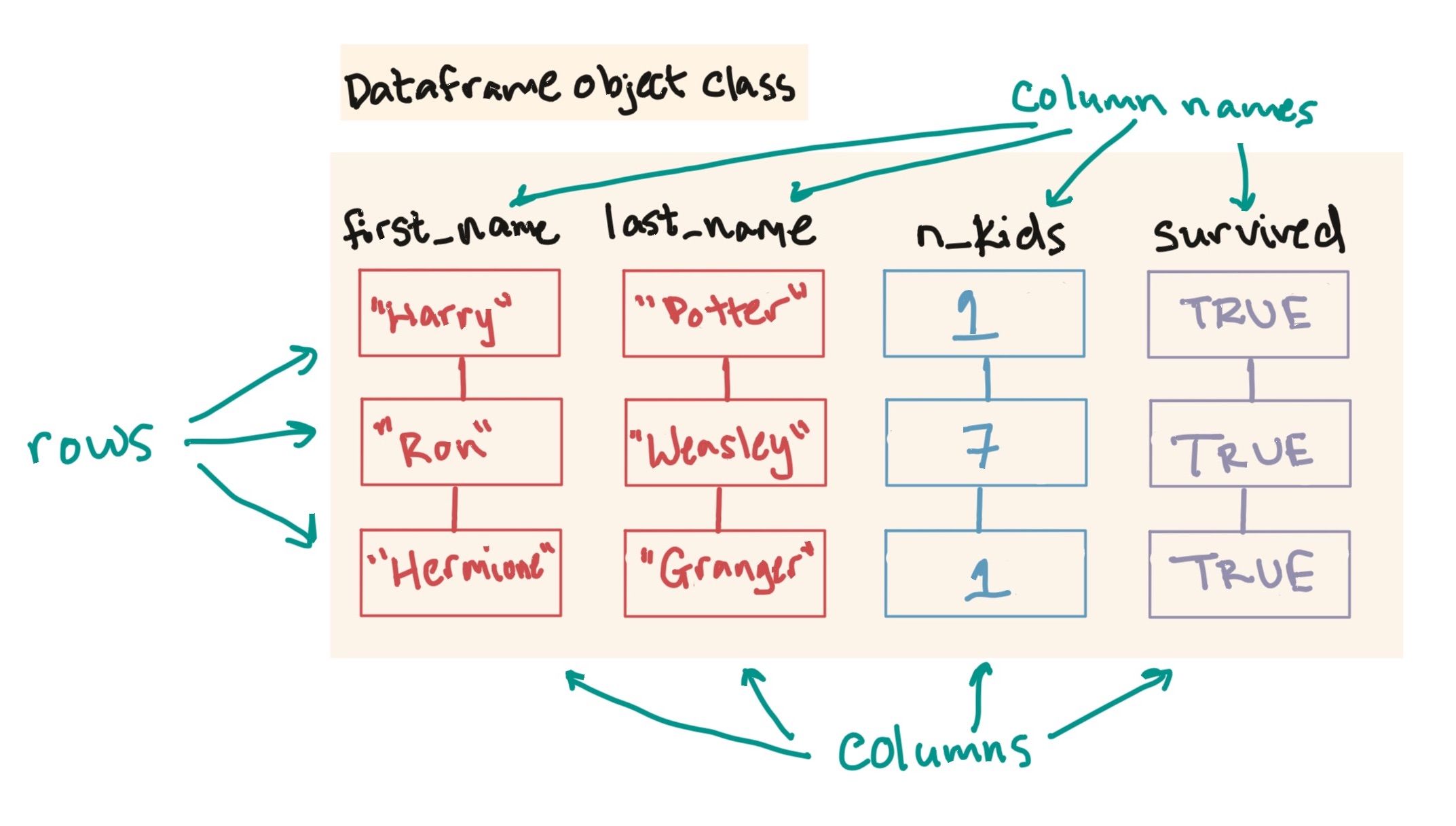
Figure 1.18: The elements of a dataframe: columns, rows, and column names.
We’ll be working with a specific class of dataframe called a tibble. You can
create tibble dataframes using the tibble function from the tibble package.
However, most often you will create a dataframe by reading in data from a file,
using something like read_csv from the readr package.
There are base R functions for both of these tasks
(data.frame and read.csv, respectively),
eliminating the need to load additional packages with a
library call. However, the series of packages that make up
what’s called the “tidyverse” have brought a huge improvement in the
ease and speed of working with data in R. We will be teaching these
tools in this course, and that’s why we’re going directly to
tibble and read_csv from the start, rather
than base R equivalents. Later in the course, we’ll talk more about this
“tidyverse” and what makes it so great.
To create a dataframe, you can use the tibble function from the tibble
package. The general format for using tibble is:
## Note: Generic code
[name of object] <- tibble([1st column name] = [1st column content],
                           [2nd column name] = [2nd column content])
with an equals sign between the column name and column content for each column, and commas between each of the columns.
Here is an example of the code used to create the Harry Potter tibble dataframe shown above:
library(package = "tibble")
hp_data <- tibble(first_name = c("Harry", "Ron", "Hermione"),
                  last_name = c("Potter", "Weasley", "Granger"),
                  n_kids = c(1, 7, 1),
                  survived = c(TRUE, TRUE, TRUE))
hp_data
## # A tibble: 3 × 4
## first_name last_name n_kids survived
## <chr> <chr> <dbl> <lgl>
## 1 Harry Potter 1 TRUE
## 2 Ron Weasley 7 TRUE
## 3 Hermione Granger 1 TRUEYou can also create a dataframe by sticking together vectors you already have saved as R objects. For example:
hp_data <- tibble(first_name = main_characters,
                  last_name = c("Potter", "Weasley", "Granger"),
                  n_kids = n_kids,
                  survived = c(TRUE, TRUE, TRUE))
hp_data
## # A tibble: 3 × 4
## first_name last_name n_kids survived
## <chr> <chr> <dbl> <lgl>
## 1 Harry Potter 1 TRUE
## 2 Ron Weasley 7 TRUE
## 3 Hermione Granger 1 TRUENote that this call requires that the main_characters and n_kids vectors are
the same length, although they don’t have to be (and in this case aren’t) the
same class of objects (main_characters is a character class, n_kids is
numeric).
You can put more than one function call in a single line of R code,
as in this example (the c creates a vector, while the
tibble creates a dataframe, using the vectors created by
the calls to c). When you use multiple functions within a
single R call, R will evaluate starting from the inner-most parentheses
out, much like the order of operations in a math equation with
parentheses.
So far, we’ve only shown how to create dataframes from scratch within an R
session. Usually, however, you’ll create R dataframes instead by reading in data
from an outside file using the read_csv from the readr package and related
functions. For example, you might want to analyze data on all the guests that
came on the Daily Show, circa Jon Stewart. If you have this data in a
comma-separated (csv) file on your computer called “daily_show_guests.csv”
(see the In-Course Exercise for instructions on downloading it), you
can read it into your R session with the following code:
In this code, the read_csv function is reading in the data from the file
“daily_show_guests.csv”, while the gets arrow (<-) assigns that data to the
object daily_show, which you can then reference in later code to explore and
plot the data.
You can use the functions dim, nrow, and ncol to figure out the dimensions
(number of rows and columns) of a dataframe:
## [1] 2693 5## [1] 2693## [1] 5Base R also has some useful functions for quickly exploring dataframes:
str: Show the structure of an R object, including a dataframesummary: Give summaries of each column of a dataframe.
For example, you can explore the data we just pulled in on the Daily Show with:
## spc_tbl_ [2,693 × 5] (S3: spec_tbl_df/tbl_df/tbl/data.frame)
##  $ YEAR                     : num [1:2693] 1999 1999 1999 1999 1999 ...
##  $ GoogleKnowlege_Occupation: chr [1:2693] "actor" "Comedian" "television actress" "film actress" ...
##  $ Show                     : chr [1:2693] "1/11/99" "1/12/99" "1/13/99" "1/14/99" ...
##  $ Group                    : chr [1:2693] "Acting" "Comedy" "Acting" "Acting" ...
##  $ Raw_Guest_List           : chr [1:2693] "Michael J. Fox" "Sandra Bernhard" "Tracey Ullman" "Gillian Anderson" ...
##  - attr(*, "spec")=
##   .. cols(
##   ..   YEAR = col_double(),
##   ..   GoogleKnowlege_Occupation = col_character(),
##   ..   Show = col_character(),
##   ..   Group = col_character(),
##   ..   Raw_Guest_List = col_character()
##   .. )
## - attr(*, "problems")=<externalptr>## YEAR GoogleKnowlege_Occupation Show Group
## Min. :1999 Length:2693 Length:2693 Length:2693
## 1st Qu.:2003 Class :character Class :character Class :character
## Median :2007 Mode :character Mode :character Mode :character
## Mean :2007
## 3rd Qu.:2011
## Max. :2015
## Raw_Guest_List
## Length:2693
## Class :character
## Mode :character
##
##
## To extract data from a dataframe, you can use some functions from the dplyr
package, select and slice. The select function will pull out columns,
while the slice function will pull out rows. In this chapter, we’ll talk about
how to extract certain rows or columns of a dataframe by their position (i.e.,
row or column number). Later in the book, we’ll talk about other ways to extract
values from dataframes.
For example, if you wanted to get the first two rows of the hp_data
dataframe, you could run:
## # A tibble: 2 × 4
##   first_name last_name n_kids survived
##   <chr>      <chr>      <dbl> <lgl>
## 1 Harry      Potter         1 TRUE
## 2 Ron        Weasley        7 TRUE
If you wanted to get the first and fourth columns, you could run:
## # A tibble: 3 × 2
##   first_name survived
##   <chr>      <lgl>
## 1 Harry      TRUE
## 2 Ron        TRUE
## 3 Hermione   TRUE
You can compose calls from both functions. For example, you could extract the values in the first and fourth columns of the first two rows with:
## # A tibble: 2 × 2
##   first_name survived
##   <chr>      <lgl>
## 1 Harry      TRUE
## 2 Ron        TRUE
You can use square-bracket indexing ([..., ...]) for dataframes, too, but now
they’ll have two dimensions (rows, then columns). Put the rows you want before
the comma, the columns after. If you want all of something (e.g., all rows in
the dataframe), leave the designated spot blank. Here are two examples of using
square-bracket indexing to pull a subset of the hp_data dataframe we
created above:
## # A tibble: 2 × 1
##   last_name
##   <chr>
## 1 Potter
## 2 Weasley## # A tibble: 1 × 4
## first_name last_name n_kids survived
## <chr> <chr> <dbl> <lgl>
## 1 Hermione Granger 1 TRUE
If you forget to put the comma in the indexing for a dataframe (e.g.,
fibonacci_seq[1:2]), you will index out the
columns that fall at that position or positions. To avoid
confusion, I suggest that you always use indexing with a comma when
working with dataframes.
Download a pdf of the lecture slides for this video.
1.10 In-course Exercise Chapter 1
You will take turns sharing your screens as you work through this exercise. Before you
start, open you R session and use the sample function, with all of your group members’
names, to randomly shuffle your names (revisit the in-course exercise in the “Course Overview”
chapter if you need a reminder).
You should do this on only one groups members computer. The order that you get from R is the order that you should take turns sharing your screen and leading the effort on coding for your group. When you are not sharing your screen, help out with suggestions, especially for general directions you could take to approach a question. (There are standards for pair programming that we’ll discuss next week, and these will provide more advice on how to productively code in a group.)
1.10.1 Trying out the code in slides for first lecture videos
Have one person in your group share their screen and take the lead in typing the code or doing the other work for this part.
To start, you’ll try running some simple code in R, using examples from the video lectures for Chapter 1. Take the following steps:
- Open an R session and find the “Console” pane.
- Go through the slides for video lectures 4 (“Function calls”) and 5 (“Objects and assignments). Find any examples of R expressions and try them out at the prompt in the console.
- Once you’ve run an assignment expression, find the “Environment” pane. Check that the object name that you assigned now appears there.
1.10.2 Writing your code as an R script
While the R console is fine for initially exploring data, you should get in the habit of writing up R code in an R script for most of your data analysis projects in R.
- Open a new R script and save it to your current working directory (i.e., wherever you saved the data you downloaded for this exercise).
- Take some of the code that you wrote for this exercise. Put it in the R script. Do not put more than one function call per line (but it’s fine to have longer function calls span a few lines).
- Use the “Run” button to run a single line of this code. Check the console to see what happens when you do.
- Highlight a few lines of the code and use “Run” to run them.
- Try using the keyboard shortcut (Command-Return) to run the line of code your cursor is currently on. Try doing this with a function call that runs across several lines of the R script file– what do you see at the console?
- Try running the whole script using “Source”. Again, look at the console after you “source” the script.
- Close your R session (and save any changes to your R script). Do not save
your R session history. Re-open R and see if you can re-open your R script and
re-run it. Try using
ls()to list the objects in your R session before and after you re-run your script. Does anything about the result surprise you?
1.10.3 About the dataset
Trade the screen sharing to the next member of your group.
For the rest of today’s class, you’ll be using a dataset of all the guests on The Daily Show when Jon Stewart was the host. This data was originally collected by Nate Silver’s website, FiveThirtyEight and is available on FiveThirtyEight’s GitHub page under the Creative Commons Attribution 4.0 International License. I have copied this data into my GitHub repository for this class. The only change made to the original file was to add (commented) attribution information at the start of the file.
First, check out a bit more about this data and its source:
- It’s often helpful to use prior knowledge to help check out or validate your dataset. One thing we might want to know about this data is if it covers the whole time that Jon Stewart hosted The Daily Show. Use Google to find out the dates he started and finished as host.
- Briefly browse around FiveThirtyEight’s GitHub data page. What are some other datasets available that you find interesting? For any dataset, you can scroll to the bottom of the page to get to the compiled README.md content, which gives the full titles and links to relevant datasets. You can also click on any dataset to get more information.
- Look at the GitHub page for this Daily Show data. How many columns will be in this dataset? What kind of information does the data include? What do the columns show? What do the rows show?
In this exercise, you’re using data posted by FiveThirtyEight on GitHub. We’ll be using a lot of data that’s on GitHub this semester, and GitHub is being used behind-the-scenes for both this book and the course note slides. We’ll talk more about GitHub later, but you might find it interesting to explore a bit now. It’s a place where people can post, work on, and share code in a number of programming languages– it’s been referred to as “Facebook for Nerds”. You can search GitHub repositories and code specifically by programming language, so it can be a good way to find example R code from which to learn.
1.10.4 Manually creating vectors
Start by manually creating some vectors and data frames with a small subset of this data.
- Use the concatenate function (
c) to create a vector “from scratch” with the names of the five guests to appear on the show (these could be the first five guests, or you could also randomly pick five guests). Assign this vector the object namefive_guests. What class (numeric or character) do you think this vector will be? Will you need to use quotation marks for each element you add to the vector? - Use square bracket indexing to print out the following subsets of this vector (you’ll have one R expression per subset): (1) The first guest in the vector; (2) The third and fifth guests; (3) The second through fourth guests.
- Create a new vector called
first_guestwith just the first guest in the vector, using the square bracket indexing you used in the previous step. - In the same way, create a vector with the year of each of these five guests’
appearances. Assign this vector to an object named
appearance_year. What class (numeric or character) do you think this vector will be? Will you need to use quotation marks for each element you add to the vector? - Use the
classfunction to determine the classes (e.g., numeric, character) of each of the vectors you just created.
Example R code:
# I picked five random guests from throughout the dataset. The guests you pick will
# likely be different.

# Create a vector with the names of five guests
five_guests <- c("Miss Piggy", "Stanley Tucci", "Kermit the Frog",
                 "Hank Azaria", "Al Gore")

# Use square-bracket indexing to print out some subsets of the data
five_guests[1]
## [1] "Miss Piggy"## [1] "Kermit the Frog" "Al Gore"## [1] "Stanley Tucci" "Kermit the Frog" "Hank Azaria"## [1] "Miss Piggy"# Create a vector with the year of the appearance of each guest
appearance_year <- c(1999, 2000, 2001, 2001, 2002)
# Figure out the classes of the two vectors you just created
class(x = five_guests)## [1] "character"## [1] "numeric"1.10.5 Installing and using a package
Trade the screen sharing to the next member of your group. Have the person who was sharing their screen save their R script and send it to this person through the Zoom chat. The new person should open this R script and use it to re-run the last part of the analysis, so that the vectors defined in the last part of the exercise can be used here.
The stringr package includes a number of functions that make it easier to work
with character strings in R. In particular, it includes functions to change the
capitalization of words in character stings. Here, you’ll install and load this
package and then use it to work with the five_guests vector we created in the
last section.
- If you have not already installed the
stringrpackage, install it from CRAN. - Load the
stringrpackage in your current R session, so you will be able to use its functions. - Check if the package has a vignette. If so, check out out that vignette.
- See if you can use the
str_to_lowerfunction from thestringrpackage to convert all the names in yourfive_guestsvector to lowercase. - See if you can find a function in the
stringrpackage that you can use to convert all the names in yourfive_guestsvector to uppercase. (Hint: At the R console, try typing?stringr::and then the Tab key.)
Example R code:
## [1] "miss piggy"      "stanley tucci"   "kermit the frog" "hank azaria"
## [5] "al gore"## [1] "MISS PIGGY" "STANLEY TUCCI" "KERMIT THE FROG" "HANK AZARIA"
## [5] "AL GORE"1.10.6 Manually creating a dataframe
- Combine the two vectors you created earlier,
five_guestsandappearance_yearto create a dataframe namedguest_list. For the columns, use the same column names used in the original, raw data for the guest names and appearance year. Print out this dataframe at the R console to make sure it looks like you thought it would. - Use functions from the
dplyrpackage to print out the following subsets of this dataframe (you’ll have one R call per subset): (1) The appearance year of the first guest; (2) Names of the third through fifth guests; (3) Names of all guests; (4) Both names and appearance years of the first and third guests. - The
strfunction can be used to figure out the structure of a dataframe. Run this command on theguest_listdataframe you created. What information does this give you? Use the helpfile forstrto help you figure this out (which you can access by running?str). Do you see anything that surprises you? - Use the
lsfunction to list all the objects you currently have defined in your R session. Compare this list to the “Environment” pane in RStudio.
Example R code:
# Create the data frame, then print it out to make sure it looks like you thought
# it would
library(package = "tibble")
guest_list <- tibble(Raw_Guest_List = five_guests,
                     YEAR = appearance_year)
guest_list
## # A tibble: 5 × 2
## Raw_Guest_List YEAR
## <chr> <dbl>
## 1 Miss Piggy 1999
## 2 Stanley Tucci 2000
## 3 Kermit the Frog 2001
## 4 Hank Azaria 2001
## 5 Al Gore 2002# Use functions from the dplyr package to extract values from the dataframe
library(package = "dplyr")
slice(.data = select(.data = guest_list, 2), 1)## # A tibble: 1 × 1
## YEAR
## <dbl>
## 1 1999## # A tibble: 3 × 1
## Raw_Guest_List
## <chr>
## 1 Kermit the Frog
## 2 Hank Azaria
## 3 Al Gore## # A tibble: 5 × 1
## Raw_Guest_List
## <chr>
## 1 Miss Piggy
## 2 Stanley Tucci
## 3 Kermit the Frog
## 4 Hank Azaria
## 5 Al Gore## # A tibble: 2 × 2
## Raw_Guest_List YEAR
## <chr> <dbl>
## 1 Miss Piggy 1999
## 2 Kermit the Frog 2001## tibble [5 × 2] (S3: tbl_df/tbl/data.frame)
## $ Raw_Guest_List: chr [1:5] "Miss Piggy" "Stanley Tucci" "Kermit the Frog" "Hank Azaria" ...
## $ YEAR : num [1:5] 1999 2000 2001 2001 20021.10.7 Getting the data onto your computer
Next, we will work with the whole dataset. Download the data from GitHub onto your computer. It is very important for you to use this link rather than downloading the data from the FiveThirtyEight GitHub page, because there’s a small difference between the two files.
In class, we created an R Project for you to use for this class. Put the Daily Show data in that directory.
Take the following steps to get the data onto your computer
- Download the file from
GitHub.
Right click on
Rawand then choose “Download linked file”. Put the file into the directory you created for this course. - Use the
list.filescommand to make sure that the “daily_show_guests.csv” file is in your current working directory (we’ll talk more about working directories, listing files in your working directory, and R Projects later in the semester).
[1] "daily_show_guests.csv"1.10.8 Getting the data into R
Now that you have the dataset in your working directory, you can read it into R.
This dataset is in a csv (comma separated values) format. (We will talk more
about different file formats in Week 2.) You can read csv files into R using the
function read_csv from the readr package.
Read the data into your R session
- If you do not already have it, install the
readrpackage. Then load this package within your current R session usinglibrary. - Use the
read_csvfunction from thereadrpackage to read the data into R and save it as the objectdaily_show(see tips in the next few bullets). - Use the help file for the
read_csvfunction to figure out how this function works. To pull that up, type?read_csvat the R console. Can you figure out why it’s critical to use theskipoption and set it to 4? (We will be talking a lot more about theread_csvfunction in Week 2, so don’t worry if you don’t completely understand it right now.) - Note that you need to put the file name in quotation marks.
- What would have happened if you’d used
read_csvbut hadn’t saved the result as the objectdaily_show? (For example, you’d run the coderead_csv("daily_show_guests.csv", skip = 4)rather thandaily_show <- read_csv("daily_show_guests.csv").)
Example R code:
# Install (if needed) and load the `readr` package
install.packages(pkgs = "readr") # You only need to do this if you
                          # do not already have the `readr`
                          # package.
library(package = "readr")

# Read in dataframe from the csv file with Daily Show guests
daily_show <- read_csv(file = "daily_show_guests.csv", skip = 4)
## Rows: 2693 Columns: 5
## ── Column specification ────────────────────────────────────────────────────────
## Delimiter: ","
## chr (4): GoogleKnowlege_Occupation, Show, Group, Raw_Guest_List
## dbl (1): YEAR
##
## ℹ Use `spec()` to retrieve the full column specification for this data.
## ℹ Specify the column types or set `show_col_types = FALSE` to quiet this message.## # A tibble: 2,693 × 5
## YEAR GoogleKnowlege_Occupation Show Group Raw_Guest_List
## <dbl> <chr> <chr> <chr> <chr>
## 1 1999 actor 1/11/99 Acting Michael J. Fox
## 2 1999 Comedian 1/12/99 Comedy Sandra Bernhard
## 3 1999 television actress 1/13/99 Acting Tracey Ullman
## 4 1999 film actress 1/14/99 Acting Gillian Anderson
## 5 1999 actor 1/18/99 Acting David Alan Grier
## 6 1999 actor 1/19/99 Acting William Baldwin
## 7 1999 Singer-lyricist 1/20/99 Musician Michael Stipe
## 8 1999 model 1/21/99 Media Carmen Electra
## 9 1999 actor 1/25/99 Acting Matthew Lillard
## 10 1999 stand-up comedian 1/26/99 Comedy David Cross
## # ℹ 2,683 more rowsIf you have extra time:
- Say this was a really big dataset. You want to check out just the first 10
rows to make sure that you’ve got your code right before you take the time to
pull in the whole dataset. Use the help file for
read_csvto figure out how to only read in a few rows. - Look through the help file for other options available for
read_csv. Can you think of examples when some of these options would be useful? - Look again at the version of this raw data on FiveThirtyEight’s GitHub page
(rather than the course’s GitHub repository, where you downloaded the data for
the course exercise). How are these two versions of the raw data different? How
would you need to change your
read_csvcall if you changed to use the FiveThirtyEight version of the raw data?
Example R code:
# Read in only the first 10 rows of the dataset
daily_show_first10 <- read_csv(file = "daily_show_guests.csv",
                       skip = 4, n_max = 10)
## Rows: 10 Columns: 5
## ── Column specification ────────────────────────────────────────────────────────
## Delimiter: ","
## chr (4): GoogleKnowlege_Occupation, Show, Group, Raw_Guest_List
## dbl (1): YEAR
##
## ℹ Use `spec()` to retrieve the full column specification for this data.
## ℹ Specify the column types or set `show_col_types = FALSE` to quiet this message.## # A tibble: 10 × 5
## YEAR GoogleKnowlege_Occupation Show Group Raw_Guest_List
## <dbl> <chr> <chr> <chr> <chr>
## 1 1999 actor 1/11/99 Acting Michael J. Fox
## 2 1999 Comedian 1/12/99 Comedy Sandra Bernhard
## 3 1999 television actress 1/13/99 Acting Tracey Ullman
## 4 1999 film actress 1/14/99 Acting Gillian Anderson
## 5 1999 actor 1/18/99 Acting David Alan Grier
## 6 1999 actor 1/19/99 Acting William Baldwin
## 7 1999 Singer-lyricist 1/20/99 Musician Michael Stipe
## 8 1999 model 1/21/99 Media Carmen Electra
## 9 1999 actor 1/25/99 Acting Matthew Lillard
## 10 1999 stand-up comedian 1/26/99 Comedy David Cross1.10.9 Checking out the data
Trade who is sharing their screen again. The new coder will need to download the data file fresh and move it into a “data” subdirectory of the R project created at the start of the class meeting. The previous coder should save and share his or her’s R script and send that to the new person by Zoom. The new person should start by running that code and making sure everything’s working well on their computer.
You now have the data available in your current R session as the daily_show
object. You’ll want to check it out to make sure it read in correctly, and also
to get a feel for the data. Throughout, you can use the help pages to figure out
more about any of the functions being used (for example, ?dim).
Take the following steps to check out the dataset
- Use the
dimfunction to find out how many rows and columns this dataframe has. Based on what you found out about the data from the GitHub page, does it have the number of columns you expected? Based on what you know about the data (that it includes all the guests who came on The Daily Show with Jon Stewart), do you think it has about the right number of rows? - Use functions from the
dplyrpackage to look at the first two rows of the dataset. Based on this, what does each row “measure” (unit of observation)? What information (variables) do you get for each “measurement”? - The
headfunction can be used to explore the first few rows of dataframes (see the helpfile at?head). Use theheadfunction to look at the first few rows of the dataframe. Does it look like the rows go in order by date? What was the date of Jon Stewart’s first show? Does it look like this dataset covers that first show? - Use the
tailfunction to look at the last few rows of the dataframe. What is the last show date covered by the dataframe? Who was the last guest?
Example R code:
# Extract values from the dataframe
library(package = "dplyr") # Load the 'dplyr' package
slice(.data = daily_show, 1:2) # Look at the first two rows of data## # A tibble: 2 × 5
## YEAR GoogleKnowlege_Occupation Show Group Raw_Guest_List
## <dbl> <chr> <chr> <chr> <chr>
## 1 1999 actor 1/11/99 Acting Michael J. Fox
## 2 1999 Comedian 1/12/99 Comedy Sandra Bernhard## [1] 2693 5## # A tibble: 6 × 5
## YEAR GoogleKnowlege_Occupation Show Group Raw_Guest_List
## <dbl> <chr> <chr> <chr> <chr>
## 1 1999 actor 1/11/99 Acting Michael J. Fox
## 2 1999 Comedian 1/12/99 Comedy Sandra Bernhard
## 3 1999 television actress 1/13/99 Acting Tracey Ullman
## 4 1999 film actress 1/14/99 Acting Gillian Anderson
## 5 1999 actor 1/18/99 Acting David Alan Grier
## 6 1999 actor 1/19/99 Acting William Baldwin## # A tibble: 6 × 5
## YEAR GoogleKnowlege_Occupation Show Group Raw_Guest_List
## <dbl> <chr> <chr> <chr> <chr>
## 1 2015 actor 7/28/15 Acting Tom Cruise
## 2 2015 biographer 7/29/15 Media Doris Kearns Goodwin
## 3 2015 director 7/30/15 Media J. J. Abrams
## 4 2015 stand-up comedian 8/3/15 Comedy Amy Schumer
## 5 2015 actor 8/4/15 Acting Denis Leary
## 6 2015 comedian 8/5/15 Comedy Louis C.K.If you have extra time:
- Say you wanted to look at the first ten rows of the dataframe, rather than the
first six. How could you use an option with
headto do this?
Example R code:
## # A tibble: 10 × 5
##     YEAR GoogleKnowlege_Occupation Show    Group    Raw_Guest_List
##    <dbl> <chr>                     <chr>   <chr>    <chr>
##  1  1999 actor                     1/11/99 Acting   Michael J. Fox
##  2  1999 Comedian                  1/12/99 Comedy   Sandra Bernhard
##  3  1999 television actress        1/13/99 Acting   Tracey Ullman
##  4  1999 film actress              1/14/99 Acting   Gillian Anderson
##  5  1999 actor                     1/18/99 Acting   David Alan Grier
##  6  1999 actor                     1/19/99 Acting   William Baldwin
##  7  1999 Singer-lyricist           1/20/99 Musician Michael Stipe
##  8  1999 model                     1/21/99 Media    Carmen Electra
##  9  1999 actor                     1/25/99 Acting   Matthew Lillard
## 10 1999 stand-up comedian 1/26/99 Comedy David Cross1.10.10 Using the data to answer questions
Nate Silver was a guest on The Daily Show. Let’s use this data to figure out how many times he was a guest and when he was on the show.
Find out more about Nate Silver on The Daily Show
(Don’t worry if you don’t make it to this sections! I’ve put it here for groups that move through the rest quickly.)
- The
filterfunction from thedplyrpackage can be combined with logical statements to help you create a specific subset of data. For example, if you only wanted data from guest visits in 1999, you could runfilter(.data = daily_show, YEAR == 1999). Check out the helpfile forfilterand use the function to create a new dataframe that only has the rows ofdaily_showwhen Nate Silver was a guest (Raw_Guest_List == "Nate Silver"). Save this as an object namednate_silver. - Print out the full
nate_silverdataframe by typingnate_silver. (You could just use this to answer both questions, but still try the next steps. They would be important with a bigger dataset.) - To count the number of times Nate Silver was a guest, you’ll need to count the
number of rows in the new dataset. You can either use the
dimfunction or thenrowfunction to do this. What additional information does thedimfunction give you? - To get the dates when Nate Silver was a guest, you can print out just the
Showcolumn of the dataframe. There are a few ways you can do this using theselectfunction from thedplyrpackage.
Example R code:
library(package = "dplyr")
# Create a subset of the data with just Nate Silver appearances
nate_silver <- filter(.data = daily_show, Raw_Guest_List == "Nate Silver")

# Investigate this subset of the data
nate_silver
## # A tibble: 3 × 5
## YEAR GoogleKnowlege_Occupation Show Group Raw_Guest_List
## <dbl> <chr> <chr> <chr> <chr>
## 1 2012 Statistician 10/17/12 Media Nate Silver
## 2 2012 Statistician 11/7/12 Media Nate Silver
## 3 2014 Statistician 3/27/14 Media Nate Silver## [1] 3 5## [1] 3## # A tibble: 3 × 1
## Show
## <chr>
## 1 10/17/12
## 2 11/7/12
## 3 3/27/14If you have extra time:
- Was Nate Silver the only statistician to be a guest on the show?
- What were the occupations that were only represented by one guest visit? Since
GoogleKnowlege_Occupationis a factor, you can use thetablefunction to create a new vector with the number of times each value ofGoogleKnowlege_Occupationshows up. You can put this information into a new vector and then pull out only the values that equal 1 (so, only had one guest). (Note that “Statistician” doesn’t show up– there was only one person who was a guest, but he had three visits.) Pick your favorite “one-off” example and find out who the guest was for that occupation.
Example R code:
statisticians <- filter(.data = daily_show,
                        GoogleKnowlege_Occupation == "Statistician")
statisticians
## # A tibble: 3 × 5
## YEAR GoogleKnowlege_Occupation Show Group Raw_Guest_List
## <dbl> <chr> <chr> <chr> <chr>
## 1 2012 Statistician 10/17/12 Media Nate Silver
## 2 2012 Statistician 11/7/12 Media Nate Silver
## 3 2014 Statistician 3/27/14 Media Nate Silvernum_visits <- table(daily_show$GoogleKnowlege_Occupation)
head(x = num_visits) # Note: This is a vector rather than a dataframe##
## - 0 academic Academic accountant activist
## 1 4 3 3 1 14single_visits <- num_visits[num_visits == 1] # This is using a "logical operator" to extract values that meet a condition
names(single_visits)## [1] "-"
## [2] "accountant"
## [3] "administrator"
## [4] "advocate"
## [5] "aei president"
## [6] "afghan politician"
## [7] "American football running back"
## [8] "american football wide reciever"
## [9] "assistant secretary of defense"
## [10] "assistant to the president for communications"
## [11] "Associate Justice of the Supreme Court of the United States"
## [12] "astronaut"
## [13] "Astronaut"
## [14] "Attorney at law"
## [15] "author of novels"
## [16] "aviator"
## [17] "Baseball athlete"
## [18] "baseball player"
## [19] "Basketball Coach"
## [20] "bass guitarist"
## [21] "bassist"
## [22] "Beach Volleyball Player"
## [23] "boxer"
## [24] "business person"
## [25] "businesswoman"
## [26] "Businesswoman"
## [27] "Cartoonist"
## [28] "celbrity chef"
## [29] "CHARACTER"
## [30] "chess player"
## [31] "chief technology officer of united states"
## [32] "Choreographer"
## [33] "civil rights activist"
## [34] "Coach"
## [35] "comic"
## [36] "Comic"
## [37] "communications consultant"
## [38] "Composer"
## [39] "comptroller of the us"
## [40] "coorespondant"
## [41] "Critic"
## [42] "designer"
## [43] "Director of the Consumer Financial Protection Bureau"
## [44] "doctor"
## [45] "drummer"
## [46] "Educator"
## [47] "entrepreneur"
## [48] "Ethologist"
## [49] "executive"
## [50] "Executive"
## [51] "fbi agent"
## [52] "Fiction writer"
## [53] "Film critic"
## [54] "film producer"
## [55] "Film-maker"
## [56] "Financier"
## [57] "first lady"
## [58] "first lady of egypt"
## [59] "First Lady of the United States"
## [60] "First Minister of Scotland"
## [61] "Football coach"
## [62] "football player"
## [63] "foreign policy analyst"
## [64] "foreign policy expert"
## [65] "foreign policy strategist"
## [66] "Former American senator"
## [67] "former british prime minister"
## [68] "former cia director"
## [69] "former director of the national economic counscil"
## [70] "Former Director of the Office of Management and Budget"
## [71] "Former First Lady of the United States"
## [72] "former governor of arizona"
## [73] "former governor of arkansas"
## [74] "former governor of california"
## [75] "Former Governor of Indiana"
## [76] "former governor of louisiana"
## [77] "former governor of massachusetts"
## [78] "former governor of michigan"
## [79] "former governor of missouri"
## [80] "former governor of montans"
## [81] "former governor of new hampshire"
## [82] "Former Governor of New Jersey"
## [83] "Former Governor of New York"
## [84] "former governor of rhode island"
## [85] "Former Governor of Texas"
## [86] "former governor of washington"
## [87] "former govrnor of masssachusetts"
## [88] "Former Mayor of Cincinnati"
## [89] "Former Mayor of New Orleans"
## [90] "former mayor of san antonio"
## [91] "Former member of the United States Senate"
## [92] "former mjority leader"
## [93] "former national security advisio\\r"
## [94] "former omb director"
## [95] "Former President of Mexico"
## [96] "Former President of the Maldives"
## [97] "former press secretary"
## [98] "former secretary of defense"
## [99] "former senator"
## [100] "former senator from kansas"
## [101] "Former United States Deputy Secretary of State"
## [102] "Former United States National Security Advisor"
## [103] "Former United States Secretary of Education"
## [104] "Former United States Secretary of Energy"
## [105] "Former United States Secretary of the Interior"
## [106] "Former United States Secretary of the Treasury"
## [107] "Former United States Secretary of Transportation"
## [108] "former us representativ"
## [109] "former us secretary of education"
## [110] "former white house counsel"
## [111] "Futurist"
## [112] "game show host"
## [113] "Geneticist"
## [114] "governor of new jersey"
## [115] "guitarist"
## [116] "high-altitude mountaineer"
## [117] "Host"
## [118] "Ice hockey coach"
## [119] "illustrator"
## [120] "Innovator"
## [121] "inspector general of homeland security department"
## [122] "intellectual"
## [123] "internet entrepreneur"
## [124] "investment banker"
## [125] "israeli official"
## [126] "JOURNALIST"
## [127] "Law professor"
## [128] "legal scholar"
## [129] "magician"
## [130] "mathematician"
## [131] "Mayor of Chicago"
## [132] "mayor of london"
## [133] "Media person"
## [134] "minister of defense"
## [135] "Music Producer"
## [136] "Neurologist"
## [137] "Neuroscientist"
## [138] "non profit director"
## [139] "non profit worker"
## [140] "orca trainer"
## [141] "pastor"
## [142] "peace activist"
## [143] "photojournalist"
## [144] "Photojournalist"
## [145] "physicist"
## [146] "pianist"
## [147] "police officer"
## [148] "political consultant"
## [149] "political expert"
## [150] "Political figure"
## [151] "political psychologist"
## [152] "political satirist"
## [153] "political strategist"
## [154] "Pop group"
## [155] "president of liberia"
## [156] "priest"
## [157] "prince"
## [158] "Product line"
## [159] "professional wrestler"
## [160] "psychic"
## [161] "Psychologist"
## [162] "public official"
## [163] "public speaker"
## [164] "publisher"
## [165] "Pundit"
## [166] "Puppeteer"
## [167] "Puzzle Creator"
## [168] "race car driver"
## [169] "Racing driver"
## [170] "reality show contestant"
## [171] "RNC chairman"
## [172] "Scholar"
## [173] "secretary of state"
## [174] "security expert"
## [175] "Soccer player"
## [176] "social activist"
## [177] "speechwriter"
## [178] "Sports Columnist"
## [179] "Surgeon"
## [180] "swimmer"
## [181] "syrian politician"
## [182] "television actor"
## [183] "television Director"
## [184] "television writer"
## [185] "televison actor"
## [186] "telvision actor"
## [187] "telvision personality"
## [188] "Tennis player"
## [189] "Track and field athlete"
## [190] "TV Producer"
## [191] "united nations official"
## [192] "United States Secretary of Agriculture"
## [193] "United States Secretary of Defense"
## [194] "United States Secretary of Housing and Urban Development"
## [195] "United States Secretary of the Navy"
## [196] "us assistant attorney"
## [197] "us official"
## [198] "us permanent representative to nato"
## [199] "us secetary of education"
## [200] "us secretary of defense"
## [201] "us secretary of energy"
## [202] "white house official"## # A tibble: 1 × 5
## YEAR GoogleKnowlege_Occupation Show Group Raw_Guest_List
## <dbl> <chr> <chr> <chr> <chr>
## 1 2012 chess player 11/8/12 Misc Katie Dellamaggiore and Pobo Ef…## # A tibble: 1 × 5
## YEAR GoogleKnowlege_Occupation Show Group Raw_Guest_List
## <dbl> <chr> <chr> <chr> <chr>
## 1 2005 mathematician 9/14/05 Academic Dr. William A. Dembski## # A tibble: 1 × 5
## YEAR GoogleKnowlege_Occupation Show Group Raw_Guest_List
## <dbl> <chr> <chr> <chr> <chr>
## 1 2015 orca trainer 3/26/15 Athletics John Hargrove## # A tibble: 1 × 5
## YEAR GoogleKnowlege_Occupation Show Group Raw_Guest_List
## <dbl> <chr> <chr> <chr> <chr>
## 1 2003 Puzzle Creator 8/20/03 Media Will Shortz## # A tibble: 1 × 5
## YEAR GoogleKnowlege_Occupation Show Group Raw_Guest_List
## <dbl> <chr> <chr> <chr> <chr>
## 1 2005 Scholar 6/13/05 Academic Larry Diamond