Chapter 2 Entering and cleaning data #1

The video lectures for this chapter are embedded at relevant places in the text, with links to download a pdf of the associated slides for each video. You can also access a full playlist for the videos for this chapter.

2.1 Objectives

After this chapter, you should (know / understand / be able to ):

Understand what a flat file is and how it differs from data stored in a binary file format
Be able to distinguish between delimited and fixed width formats for flat files
Be able to identify the delimiter in a delimited file
Be able to describe a working directory
Be able to read in different types of flat files
Be able to read in a few types of binary files (SAS, Excel)
Understand the difference between relative and absolute file pathnames
Describe the basics of your computer’s directory structure
Reference files in different locations in your directory structure using relative and absolute pathnames
Use the basic dplyr functions rename, select, mutate, slice, filter, and arrange to work with data in a dataframe object
Convert a column to a date format using lubridate functions
Extract information from a date object (e.g., month, year, day of week) using lubridate functions
Define a logical operator and know the R syntax for common logical operators
Use logical operators in conjunction with dplyr’s filter function to create subsets of a dataframe based on logical conditions
Use piping to apply multiple dplyr functions in sequence to a dataframe

2.2 Overview

Download a pdf of the lecture slides for this video.

There are four basic steps you will often repeat as you prepare to analyze data in R:

Identify where the data is (If it’s on your computer, which directory? If it’s online, what’s the url?)
Read data into R (e.g., read_delim, read_csv from the readr package) using the file path you figured out in step 1
Check to make sure the data came in correctly (dim, head, tail, str)
Clean the data up

In this chapter, I’ll go basics for each of these steps, as well as dive a bit deeper into some related topics you should learn now to make your life easier as you get started using R for research.

2.3 Reading data into R

Data comes in files of all shapes and sizes. R has the capability to read data in from many of these, even proprietary files for other software (e.g., Excel and SAS files). As a small sample, here are some of the types of data files that R can read and work with:

Flat files (much more about these in just a minute)
Files from other statistical packages (SAS, Excel, Stata, SPSS)
Tables on webpages (e.g., the table on ebola outbreaks near the end of this Wikipedia page)
Data in a database (e.g., MySQL, Oracle)
Data in JSON and XML formats
Really crazy data formats used in other disciplines (e.g., netCDF files from climate research, MRI data stored in Analyze, NIfTI, and DICOM formats)
Geographic shapefiles
Data through APIs

Often, it is possible to read in and clean up even incredibly messy data, by using functions like scan and readLines to read the data in a line at a time, and then using regular expressions (which I’ll cover in the “Intermediate” section of the course) to clean up each line as it comes in. In over a decade of coding in R, I think the only time I’ve come across a data file I couldn’t get into R was for proprietary precision agriculture data collected at harvest by a combine.

2.3.1 Reading local flat files

Much of the data that you will want to read in will be in flat files. Basically, these are files that you can open using a text editor; the most common type you’ll work with are probably comma-separated files (often with a .csv or .txt file extension). Most flat files come in two general categories:

Fixed width files; and
Delimited files:

“.csv”: Comma-separated values
“.tab”, “.tsv”: Tab-separated values
Other possible delimiters: colon, semicolon, pipe (“|”)

Fixed width files are files where a column always has the same width, for all the rows in the column. These tend to look very neat and easy-to-read when you open them in a text editor. For example, the first few rows of a fixed-width file might look like this:

Course            Number          Day          Time
Intro to Epi      501             M/W/F        9:00-9:50
Advanced Epi      521             T/Th         1:00-2:15

Fixed width files used to be very popular, and they make it easier to look at data when you open the file in a text editor. However, now it’s pretty rare to just use a text editor to open a file and check out the data, and these files can be a bit of a pain to read into R and other programs because you sometimes have to specify exactly how wide each of the columns is. You may come across a fixed width file every now and then, though, particularly when working with older data sets, so it’s useful to be able to recognize one and to know how to read it in.

Delimited files use some delimiter (for example, a column or a tab) to separate each column value within a row. The first few rows of a delimited file might look like this:

Course, Number, Day, Time
"Intro to Epi", 501, "M/W/F", "9:00-9:50"
"Advanced Epi", 521, "T/Th", "1:00-2:15"

Delimited files are very easy to read into R. You just need to be able to figure out what character is used as a delimiter (commas in the example above) and specify that to R in the function call to read in the data.

These flat files can have a number of different file extensions. The most generic is .txt, but they will also have ones more specific to their format, like .csv for a comma-delimited file or .fwf for a fixed with file.

Download a pdf of the lecture slides for this video.

R can read in data from both fixed with and delimited flat files. The only catch is that you need to tell R a bit more about the format of the flat file, including whether it is fixed width or delimited. If the file is fixed width, you will usually have to tell R the width of each column. If the file is delimited, you’ll need to tell R which delimiter is being used.

If the file is delimited, you can use the read_delim family of functions from the readr package to read it in. This family of functions includes several specialized functions. All members of the read_delim family are doing the same basic thing. The only difference is what defaults each function has for the delimiter (delim). Members of the read_delim family include:

Function	Delimiter
`read_csv`	comma
`read_csv2`	semi-colon
`read_table2`	whitespace
`read_tsv`	tab

You can use read_delim to read in any delimited file, regardless of the delimiter. However, you will need to specify the delimiter using the delim parameters. If you remember the more specialized function call (e.g., read_csv for a comma delimited file), therefore, you can save yourself some typing.

For example, to read in the Ebola data, which is comma-delimited, you could either use read_table with a delim argument specified or use read_csv, in which case you don’t have to specify delim:

library(package = "readr")

# The following two calls do the same thing
ebola <- read_delim(file = "data/country_timeseries.csv", delim = ",")

ebola <- read_csv(file = "data/country_timeseries.csv")

## Rows: 122 Columns: 18
## ── Column specification ────────────────────────────────────────────────────────
## Delimiter: ","
## chr  (1): Date
## dbl (17): Day, Cases_Guinea, Cases_Liberia, Cases_SierraLeone, Cases_Nigeria...
## 
## ℹ Use `spec()` to retrieve the full column specification for this data.
## ℹ Specify the column types or set `show_col_types = FALSE` to quiet this message.

The message that R prints after this call (“Parsed with column specification:..”) lets you know what classes were used for each column (this function tries to guess the appropriate class and typically gets it right). You can suppress the message using the cols_types = cols() argument.

If readr doesn’t correctly guess some of the columns classes you can use the type_convert() function to take another go at guessing them after you’ve tweaked the formats of the rogue columns.

This family of functions has a few other helpful options you can specify. For example, if you want to skip the first few lines of a file before you start reading in the data, you can use skip to set the number of lines to skip. If you only want to read in a few lines of the data, you can use the n_max option. For example, if you have a really long file, and you want to save time by only reading in the first ten lines as you figure out what other options to use in read_delim for that file, you could include the option n_max = 10 in the read_delim call. Here is a table of some of the most useful options common to the read_delim family of functions:

Option	Description
`skip`	How many lines of the start of the file should you skip?
`col_names`	What would you like to use as the column names?
`col_types`	What would you like to use as the column types?
`n_max`	How many rows do you want to read in?
`na`	How are missing values coded?

Remember that you can always find out more about a function by looking at its help file. For example, check out ?read_delim and ?read_fwf. You can also use the help files to determine the default values of arguments for each function.

So far, we’ve only looked at functions from the readr package for reading in data files. There is a similar family of functions available in base R, the read.table family of functions. The readr family of functions is very similar to the base R read.table functions, but have some more sensible defaults. Compared to the read.table family of functions, the readr functions:

Work better with large datasets: faster, includes progress bar
Have more sensible defaults (e.g., characters default to characters, not factors)

I recommend that you always use the readr functions rather than their base R alternatives, given these advantages. However, you are likely to come across code that someone else has written that uses one of these base R functions, so it’s helpful to know what they are. Functions in the read.table family include:

read.csv
read.delim
read.table
read.fwf

The readr package is a member of the tidyverse of packages. The tidyverse describes an evolving collection of R packages with a common philosophy, and they are unquestionably changing the way people code in R. Many were developed in part or full by Hadley Wickham and others at RStudio. Many of these packages are less than ten years old, but have been rapidly adapted by the R community. As a result, newer examples of R code will often look very different from the code in older R scripts, including examples in books that are more than a few years old. In this course, I’ll focus on “tidyverse” functions when possible, but I do put in details about base R equivalent functions or processes at some points—this will help you interpret older code. You can download all the tidyverse packages using install.packages(“tidyverse”), library(“tidyverse”) makes all the tidyverse functions available for use.

2.3.2 Reading in other file types

Later in the course, we’ll talk about how to open a variety of other file types in R. However, you might find it immediately useful to be able to read in files from other statistical programs.

There are two “tidyverse” packages—readxl and haven—that help with this. They allow you to read in files from the following formats:

File type	Function	Package
Excel	`read_excel`	`readxl`
SAS	`read_sas`	`haven`
SPSS	`read_spss`	`haven`
Stata	`read_stata`	`haven`

2.4 Directories and pathnames

2.4.1 Directory structure

Download a pdf of the lecture slides for this video.

So far, we’ve only looked at reading in files that are located in your current working directory. For example, if you’re working in an R Project, by default the project will open with that directory as the working directory, so you can read files that are saved in that project’s main directory using only the file name as a reference.

However, you’ll often want to read in files that are located somewhere else on your computer, or even files that are saved on another computer (for example, data files that are posted online). Doing this is very similar to reading in a file that is in your current working directory; the only difference is that you need to give R some directions so it can find the file.

The most common case will be reading in files in a subdirectory of your current working directory. For example, you may have created a “data” subdirectory in one of your R Projects directories to keep all the project’s data files in the same place while keeping the structure of the main directory fairly clean. In this case, you’ll need to direct R into that subdirectory when you want to read one of those files.

To understand how to give R these directions, you need to have some understanding of the directory structure of your computer. It seems a bit of a pain and a bit complex to have to think about computer directory structure in the “basics” part of this class, but this structure is not terribly complex once you get the idea of it. There are a couple of very good reasons why it’s worth learning now.

First, many of the most frustrating errors you get when you start using R trace back to understanding directories and filepaths. For example, when you try to read a file into R using only the filename, and that file is not in your current working directory, you will get an error like:

Error in file(file, "rt") : cannot open the connection
In addition: Warning message:
In file(file, "rt") : cannot open file 'Ex.csv': No such file or directory

This error is especially frustrating when you’re new to R because it happens at the very beginning of your analysis—you can’t even get your data in. Also, if you don’t understand a bit about working directories and how R looks for the file you’re asking it to find, you’d have no idea where to start to fix this error. Second, once you understand how to use pathnames, especially relative pathnames, to tell R how to find a file that is in a directory other than your working directory, you will be able to organize all of your files for a project in a much cleaner way. For example, you can create a directory for your project, then create one subdirectory to store all of your R scripts, and another to store all of your data, and so on. This can help you keep very complex projects more structured and easier to navigate. We’ll talk about these ideas more in the course sections on Reproducible Research, but it’s good to start learning how directory structures and filepaths work early.

Your computer organizes files through a collection of directories. Chances are, you are fairly used to working with these in your daily life already (although you may call them “folders” rather than “directories”). For example, you’ve probably created new directories to store data files and Word documents for a specific project.

Figure 2.1 gives an example file directory structure for a hypothetical computer. Directories are shown in blue, and files in green.

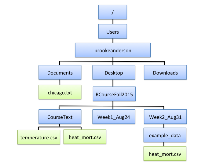
Figure 2.1: An example of file directory structure.

You can notice a few interesting things from Figure 2.1. First, you might notice the structure includes a few of the directories that you use a lot on your own computer, like Desktop, Documents, and Downloads. Next, the directory at the very top is the computer’s root directory, /. For a PC, the root directory might something like C:; for Unix and Macs, it’s usually /. Finally, if you look closely, you’ll notice that it’s possible to have different files in different locations of the directory structure with the same file name. For example, in the figure, there are files names heat_mort.csv in both the CourseText directory and in the example_data directory. These are two different files with different contents, but they can have the same name as long as they’re in different directories. This fact—that you can have files with the same name in different places—should help you appreciate how useful it is that R requires you to give very clear directions to describe exactly which file you want R to read in, if you aren’t reading in something in your current working directory.

You will have a home directory somewhere near the top of your structure, although it’s likely not your root directory. In the hypothetic computer in Figure 2.1, the home directory is /Users/brookeanderson. I’ll describe just a bit later how you can figure out what your own home directory is on your own computer.

2.4.2 Working directory

When you run R, it’s always running from within some working directory, which will be one of the directories somewhere in your computer’s directory structure. At any time, you can figure out which directory R is working in by running the command getwd() (short for “get working directory”). For example, my R session is currently running in the following directory:

getwd()

## [1] "C:/Users/rseverso/Documents/RProgrammingForResearch"

This means that, for my current R session, R is working in the RProgrammingForResearch subdirectory of my brookeanderson directory (which is my home directory).

There are a few general rules for which working directory R will start in when you open an R session. These are not absolute rules, but they’re generally true. If you have R closed, and you open it by double-clicking on an R script, then R will generally open with, as its working directory, the directory in which that script is stored. This is often a very convenient convention, because often any of the data you’ll be reading in for that script is somewhere near where the script file is saved in the directory structure. If you open R by double-clicking on the R icon in “Applications” (or something similar on a PC), R will start in its default working directory. You can find out what this is, or change it, in RStudio’s “Preferences”. Finally, if you open an R Project, R will start in that project’s working directory (the directory in which the .Rproj file for the project is stored).

2.4.3 File and directory pathnames

Download a pdf of the lecture slides for this video.

Once you get a picture of how your directories and files are organized, you can use pathnames, either absolute or relative, to read in files from different directories than your current working directory. Pathnames are the directions for getting to a directory or file stored on your computer.

When you want to reference a directory or file, you can use one of two types of pathnames:

Relative pathname: How to get to the file or directory from your current working directory
Absolute pathname: How to get to the file or directory from anywhere on the computer

Absolute pathnames are a bit more straightforward conceptually, because they don’t depend on your current working directory. However, they’re also a lot longer to write, and they’re much less convenient if you’ll be sharing some of your code with other people who might run it on their own computers. I’ll explain this second point a bit more later in this section.

Absolute pathnames give the full directions to a directory or file, starting all the way at the root directory. For example, the heat_mort.csv file in the CourseText directory has the absolute pathname:

"/Users/brookeanderson/Desktop/RCourseFall2015/CourseText/heat_mort.csv"

You can use this absolute pathname to read this file in using any of the readr functions to read in data. This absolute pathname will always work, regardless of your current working directory, because it gives directions from the root—it will always be clear to R exactly what file you’re talking about. Here’s the code to use to read that file in using the read.csv function with the file’s absolute pathname:

heat_mort <- read_csv(file = "/Users/brookeanderson/Desktop/RCourseFall2015/CourseText/heat_mort.csv")

The relative pathname, on the other hand, gives R the directions for how to get to a directory or file from the current working directory. If the file or directory you’re looking for is pretty close to your current working directory in your directory structure, then a relative pathname can be a much shorter way to tell R how to get to the file than an absolute pathname. However, the relative pathname depends on your current working directory—the relative pathname that works perfectly when you’re working in one directory will not work at all once you move into a different working directory.

As an example of a relative pathname, say you’re working in the directory RCourseFall2015 within the file structure shown in Figure 2.1, and you want to read in the heat_mort.csv file in the CourseText directory. To get from RCourseFall2015 to that file, you’d need to look in the subdirectory CourseText, where you could find heat_mort.csv. Therefore, the relative pathname from your working directory would be:

"CourseText/heat_mort.csv"

You can use this relative pathname to tell R where to find and read in the file:

heat_mort <- read_csv("CourseText/heat_mort.csv")

While this pathname is much shorter than the absolute pathname, it is important to remember that if you are working in a different working directory, this relative pathname would no longer work.

There are a few abbreviations that can be really useful for pathnames:

Shorthand	Meaning
`~`	Home directory
`.`	Current working directory
`..`	One directory up from current working directory
`../..`	Two directories up from current working directory

These can help you keep pathnames shorter and also help you move “up-and-over” to get to a file or directory that’s not on the direct path below your current working directory.

For example, my home directory is /Users/brookeanderson. You can use the list.files() function to list all the files in a directory. If I wanted to list all the files in my Downloads directory, which is a direct sub-directory of my home directory, I could use:

list.files("~/Downloads")

As a second example, say I was working in the working directory CourseText, but I wanted to read in the heat_mort.csv file that’s in the example_data directory, rather than the one in the CourseText directory. I can use the .. abbreviation to tell R to look up one directory from the current working directory, and then down within a subdirectory of that. The relative pathname in this case is:

"../Week2_Aug31/example_data/heat_mort.csv"

This tells R to look one directory up from the working directory (..) (this is also known as the parent directory of the current directory), which in this case is to RCourseFall2015, and then down within that directory to Week2_Aug31, then to example_data, and then to look there for the file heat_mort.csv.

The relative pathname to read this file while R is working in the CourseTest directory would be:

heat_mort <- read_csv("../Week2_Aug31/example_data/heat_mort.csv")

Relative pathnames “break” as soon as you tried them from a different working directory—this fact might make it seem like you would never want to use relative pathnames, and would always want to use absolute ones instead, even if they’re longer. If that were the only consideration (length of the pathname), then perhaps that would be true. However, as you do more and more in R, there will likely be many occasions when you want to use relative pathnames instead. They are particularly useful if you ever want to share a whole directory, with all subdirectories, with a collaborator. In that case, if you’ve used relative pathnames, all the code should work fine for the person you share with, even though they’re running it on their own computer. Conversely, if you’d used absolute pathnames, none of them would work on another computer, because the “top” of the directory structure (i.e., for me, /Users/brookeanderson/Desktop) will almost definitely be different for your collaborator’s computer than it is for yours.

If you’re getting errors reading in files, and you think it’s related to the relative pathname you’re using, it’s often helpful to use list.files() to make sure the file you’re trying to load is in the directory that the relative pathname you’re using is directing R to.

2.4.4 Diversion: `paste`

This is a good opportunity to explain how to use some functions that can be very helpful when you’re using relative or absolute pathnames: paste() and paste0().

As a bit of important background information, it’s important that you understand that you can save a pathname (absolute or relative) as an R object, and then use that R object in calls to later functions like list.files() and read_csv(). For example, to use the absolute pathname to read the heat_mort.csv file in the CourseText directory, you could run:

my_file <- "/Users/brookeanderson/Desktop/RCourseFall2015/CourseText/heat_mort.csv"
heat_mort <- read_csv(file = my_file)

You’ll notice from this code that the pathname to get to a directory or file can sometimes become ungainly and long. To keep your code cleaner, you can address this by using the paste or paste0 functions. These functions come in handy in a lot of other applications, too, but this is a good place to introduce them.

The paste() function is very straightforward. It takes, as inputs, a series of different character strings you want to join together, and it pastes them together in a single character string. (As a note, this means that your result vector will only be one element long, for basic uses of paste(), while the inputs will be several different character stings.) You separate all the different things you want to paste together using with commas in the function call. For example:

paste("Sunday", "Monday", "Tuesday")

## [1] "Sunday Monday Tuesday"

length(x = c("Sunday", "Monday", "Tuesday"))

## [1] 3

length(x = paste("Sunday", "Monday", "Tuesday"))

## [1] 1

The paste() function has an option called sep =. This tells R what you want to use to separate the values you’re pasting together in the output. The default is for R to use a space, as shown in the example above. To change the separator, you can change this option, and you can put in just about anything you want. For example, if you wanted to paste all the values together without spaces, you could use sep = "":

paste("Sunday", "Monday", "Tuesday", sep = "")

## [1] "SundayMondayTuesday"

As a shortcut, instead of using the sep = "" option, you could achieve the same thing using the paste0 function. This function is almost exactly like paste, but it defaults to "" (i.e., no space) as the separator between values by default:

paste0("Sunday", "Monday", "Tuesday")

## [1] "SundayMondayTuesday"

With pathnames, you will usually not want spaces. Therefore, you could think about using paste0() to write an object with the pathname you want to ultimately use in commands like list.files() and setwd(). This will allow you to keep your code cleaner, since you can now divide long pathnames over multiple lines:

my_file <- paste0("/Users/brookeanderson/Desktop/",
                  "RCourseFall2015/CourseText/heat_mort.csv")
heat_mort <- read_csv(file = my_file)

You will end up using paste() and paste0() for many other applications, but this is a good example of how you can start using these functions to start to get a feel for them.

2.4.5 Reading online flat files

So far, I’ve only shown you how to read in data from files that are saved to your computer. R can also read in data directly from the web. If a flat file is posted online, you can read it into R in almost exactly the same way that you would read in a local file. The only difference is that you will use the file’s url instead of a local file path for the file argument.

With the read_* family of functions, you can do this both for flat files from a non-secure webpage (i.e., one that starts with http) and for files from a secure webpage (i.e., one that starts with https), including GitHub and Dropbox.

For example, to read in data from this GitHub repository of Ebola data, you can run:

library("dplyr")
url <- paste0("https://raw.githubusercontent.com/cmrivers/",
              "ebola/master/country_timeseries.csv")
ebola <- read_csv(file = url)
slice(.data = (select(.data = ebola, 1:3)), 1:3)

## # A tibble: 3 × 3
##   Date       Day Cases_Guinea
##   <chr>    <dbl>        <dbl>
## 1 1/5/2015   289         2776
## 2 1/4/2015   288         2775
## 3 1/3/2015   287         2769

2.5 Data cleaning

Download a pdf of the lecture slides for this video.

Once you have loaded data into R, you’ll likely need to clean it up a little before you’re ready to analyze it. Here, I’ll go over the first steps of how to do that with functions from dplyr, another package in the tidyverse. Here are some of the most common data-cleaning tasks, along with the corresponding dplyr function for each:

Task	`dplyr` function
Renaming columns	`rename`
Filtering to certain rows	`filter`
Selecting certain columns	`select`
Adding or changing columns	`mutate`

In this section, I’ll describe how to do each of these tasks; in later sections of the course, we’ll go much deeper into how to clean messier data.

For the examples in this section, I’ll use example data listing guests to the Daily Show. To follow along with these examples, you’ll want to load that data, as well as load the dplyr package (install it using install.packages if you have not already):

library("dplyr")
daily_show <- read_csv(file = "data/daily_show_guests.csv", skip = 4)

I’ve used this data in previous examples, but as a reminder, here’s what it looks like:

head(x = daily_show)

## # A tibble: 6 × 5
##    YEAR GoogleKnowlege_Occupation Show    Group  Raw_Guest_List  
##   <dbl> <chr>                     <chr>   <chr>  <chr>           
## 1  1999 actor                     1/11/99 Acting Michael J. Fox  
## 2  1999 Comedian                  1/12/99 Comedy Sandra Bernhard 
## 3  1999 television actress        1/13/99 Acting Tracey Ullman   
## 4  1999 film actress              1/14/99 Acting Gillian Anderson
## 5  1999 actor                     1/18/99 Acting David Alan Grier
## 6  1999 actor                     1/19/99 Acting William Baldwin

2.5.1 Renaming columns

A first step is often re-naming the columns of the dataframe. It can be hard to work with a column name that:

is long
includes spaces or other special characters
includes upper case

You can check out the column names for a dataframe using the colnames function, with the dataframe object as the argument. Several of the column names in daily_show have some of these issues:

colnames(x = daily_show)

## [1] "YEAR"                      "GoogleKnowlege_Occupation"
## [3] "Show"                      "Group"                    
## [5] "Raw_Guest_List"

To rename these columns, use rename. The basic syntax is:

## Generic code
rename(.data = dataframe, 
       new_column_name_1 = old_column_name_1,
       new_column_name_2 = old_column_name_2)

The first argument is the dataframe for which you’d like to rename columns. Then you list each pair of new versus old column names (in that order) for each of the columns you want to rename. To rename columns in the daily_show data using rename, for example, you would run:

daily_show <- rename(.data = daily_show,
                     year = YEAR,
                     job = GoogleKnowlege_Occupation, 
                     date = Show, 
                     category = Group,
                     guest_name = Raw_Guest_List)
head(x = daily_show, 3)

## # A tibble: 3 × 5
##    year job                date    category guest_name     
##   <dbl> <chr>              <chr>   <chr>    <chr>          
## 1  1999 actor              1/11/99 Acting   Michael J. Fox 
## 2  1999 Comedian           1/12/99 Comedy   Sandra Bernhard
## 3  1999 television actress 1/13/99 Acting   Tracey Ullman

Many of the functions in tidyverse packages, including those in dplyr, provide exceptions to the general rule about when to use quotation marks versus when to leave them off. Unfortunately, this may make it a bit hard to learn when to use quotation marks versus when not to. One way to think about this, which is a bit of an oversimplification but can help as you’re learning, is to assume that anytime you’re using a dplyr function, every column in the dataframe you’re working with has been loaded to your R session as its own object.

2.5.2 Selecting columns

Download a pdf of the lecture slides for this video.

Next, you may want to select only some columns of the dataframe. You can use the select function from dplyr to subset the dataframe to certain columns. The basic structure of this command is:

## Generic code
select(.data = dataframe, column_name_1, column_name_2, ...)

In this call, you first specify the dataframe to use and then list all of the column names to include in the output dataframe, with commas between each column name. For example, to select all columns in daily_show except year (since that information is already included in date), run:

select(.data = daily_show, job, date, category, guest_name)

## # A tibble: 2,693 × 4
##    job                date    category guest_name      
##    <chr>              <chr>   <chr>    <chr>           
##  1 actor              1/11/99 Acting   Michael J. Fox  
##  2 Comedian           1/12/99 Comedy   Sandra Bernhard 
##  3 television actress 1/13/99 Acting   Tracey Ullman   
##  4 film actress       1/14/99 Acting   Gillian Anderson
##  5 actor              1/18/99 Acting   David Alan Grier
##  6 actor              1/19/99 Acting   William Baldwin 
##  7 Singer-lyricist    1/20/99 Musician Michael Stipe   
##  8 model              1/21/99 Media    Carmen Electra  
##  9 actor              1/25/99 Acting   Matthew Lillard 
## 10 stand-up comedian  1/26/99 Comedy   David Cross     
## # ℹ 2,683 more rows

Don’t forget that, if you want to change column names in the saved object, you must reassign the object to be the output of rename. If you run one of these cleaning functions without reassigning the object, R will print out the result, but the object itself won’t change. You can take advantage of this, as I’ve done in this example, to look at the result of applying a function to a dataframe without changing the original dataframe. This can be helpful as you’re figuring out how to write your code.

The select function also provides some time-saving tools. For example, in the last example, we wanted all the columns except one. Instead of writing out all the columns we want, we can use - with the columns we don’t want to save time:

daily_show <- select(.data = daily_show, -year)
head(x = daily_show, n = 3)

## # A tibble: 3 × 4
##   job                date    category guest_name     
##   <chr>              <chr>   <chr>    <chr>          
## 1 actor              1/11/99 Acting   Michael J. Fox 
## 2 Comedian           1/12/99 Comedy   Sandra Bernhard
## 3 television actress 1/13/99 Acting   Tracey Ullman

2.5.3 Extracting and arranging rows

Download a pdf of the lecture slides for this video.

There are a number of different actions you can take to extract or rearrange rows from a dataset to clean it up for your current analysis, including:

slice
sample_n
arrange
filter

We’ll go through what each of these does and how to use them.

2.5.4 Slicing and sampling

The slice function from the dplyr package can extract certain rows based on their position in the dataframe.

We already looked at this a bit in Chapter 1. In the last chapter, you learned how to use the slice function to limit a dataframe to certain rows by row position.

For example, to print the first three rows of the daily_show data, you can run:

library("dplyr")
slice(.data = daily_show, 1:3)

## # A tibble: 3 × 4
##   job                date    category guest_name     
##   <chr>              <chr>   <chr>    <chr>          
## 1 actor              1/11/99 Acting   Michael J. Fox 
## 2 Comedian           1/12/99 Comedy   Sandra Bernhard
## 3 television actress 1/13/99 Acting   Tracey Ullman

There are some other functions you can use to extract rows from a tibble dataframe, all from the “dplyr” package.

For example, if you’d like to extract a random subset of n rows, you can use the sample_n function, with the size argument set to n.

To extract two random rows from the daily_show dataframe, run:

sample_n(tbl = daily_show, size = 2)

## # A tibble: 2 × 4
##   job       date    category guest_name   
##   <chr>     <chr>   <chr>    <chr>        
## 1 Filmmaker 6/7/00  Media    Michael Moore
## 2 author    2/13/08 Media    Mark Siegel

2.5.5 Arranging rows

There is also a function, arrange, you can use to re-order the rows in a dataframe based on the values in one of its columns. The syntax for this function is:

# Generic code
arrange(.data = dataframe, column_to_order_by)

If you run this function to use a character vector to order, it will order the rows alphabetically by the values in that column. If you specify a numeric vector, it will order the rows by the numeric value.

For example, we could reorder the daily_show data alphabetically by the values in the category column with the following call:

daily_show <- arrange(.data = daily_show, category)
slice(.data = daily_show, 1:3)

## # A tibble: 3 × 4
##   job       date    category guest_name       
##   <chr>     <chr>   <chr>    <chr>            
## 1 professor 10/3/01 Academic Stephen S. Morse 
## 2 Professor 12/3/01 Academic Nadine Strossen  
## 3 Historian 11/4/03 Academic Michael Beschloss

If you want the ordering to be reversed (e.g., from “z” to “a” for character vectors, from higher to lower for numeric, latest to earliest for a Date), you can include the desc function.

For example, to reorder the daily_show data by job category in descending alphabetical order, you can run:

daily_show <- arrange(.data = daily_show, 
                      desc(x = category))
slice(.data = daily_show, 1:2)

## # A tibble: 2 × 4
##   job         date     category guest_name   
##   <chr>       <chr>    <chr>    <chr>        
## 1 news anchor 3/21/01  media    Jeff Varner  
## 2 news anchor 10/15/02 media    Judy Woodruff

2.5.6 Filtering to certain rows

Next, you might want to filter the dataset down so that it only includes certain rows. For example, you might want to get a dataset with only the guests from 2015, or only guests who are scientists.

You can use the filter function from dplyr to filter a dataframe down to a subset of rows. The syntax is:

## Generic code
filter(.data = dataframe, logical expression)

The logical expression in this call gives the condition that a row must meet to be included in the output data frame. For example, if you want to create a data frame that only includes guests who were scientists, you can run:

scientists <- filter(.data = daily_show, 
                     category == "Science")
head(x = scientists)

## # A tibble: 6 × 4
##   job            date    category guest_name            
##   <chr>          <chr>   <chr>    <chr>                 
## 1 neurosurgeon   4/28/03 Science  Dr Sanjay Gupta       
## 2 scientist      1/13/04 Science  Catherine Weitz       
## 3 physician      6/15/04 Science  Hassan Ibrahim        
## 4 doctor         9/6/05  Science  Dr. Marc Siegel       
## 5 astronaut      2/13/06 Science  Astronaut Mike Mullane
## 6 Astrophysicist 1/30/07 Science  Neil deGrasse Tyson

To build a logical expression to use in filter, you’ll need to know some of R’s logical operators. Some of the most commonly used ones are:

Operator	Meaning	Example
`==`	equals	`category == "Acting"`
`!=`	does not equal	`category != "Comedy"`
`%in%`	is in	`category %in% c("Academic", "Science")`
`is.na()`	is missing	`is.na(job)`
`!is.na()`	is not missing	`!is.na(job)`
`&`	and	`year == 2015 & category == "Academic"`
`\|`	or	`year == 2015 \| category == "Academic"`

We’ll use these logical operators and expressions a lot more as the course continues, so they’re worth learning by heart.

Two common errors with logical operators are: (1) Using = instead of == to check if two values are equal; and (2) Using == NA instead of is.na to check for missing observations.

2.5.7 Add or change columns

Download a pdf of the lecture slides for this video.

You can change a column or add a new column using the mutate function from the dplyr package. That function has the syntax:

# Generic code
mutate(.data = dataframe,
       changed_column = function(changed_column),
       new_column = function(other arguments))

For example, the job column in daily_show sometimes uses upper case and sometimes does not (this call uses the unique function to list only unique values in this column):

head(x = unique(x = daily_show$job), n = 10)

##  [1] "news anchor"    "neurosurgeon"   "scientist"      "physician"     
##  [5] "doctor"         "astronaut"      "Astrophysicist" "Surgeon"       
##  [9] "Neuroscientist" "primatologist"

To make all the observations in the job column lowercase, use the str_to_lower function from the stringr package within a mutate function:

library(package = "stringr")
mutate(.data = daily_show, 
       job = str_to_lower(string = job))

## # A tibble: 2,693 × 4
##    job          date     category guest_name            
##    <chr>        <chr>    <chr>    <chr>                 
##  1 news anchor  3/21/01  media    Jeff Varner           
##  2 news anchor  10/15/02 media    Judy Woodruff         
##  3 news anchor  11/6/02  media    Candy Crowley         
##  4 news anchor  4/9/02   media    Judy Woodruff         
##  5 news anchor  3/24/11  media    Bret Baier            
##  6 neurosurgeon 4/28/03  Science  Dr Sanjay Gupta       
##  7 scientist    1/13/04  Science  Catherine Weitz       
##  8 physician    6/15/04  Science  Hassan Ibrahim        
##  9 doctor       9/6/05   Science  Dr. Marc Siegel       
## 10 astronaut    2/13/06  Science  Astronaut Mike Mullane
## # ℹ 2,683 more rows

2.6 Piping

Download a pdf of the lecture slides for this video.

So far, I’ve shown how to use these dplyr functions one at a time to clean up the data, reassigning the dataframe object at each step. However, there’s a trick called “piping” that will let you clean up your code a bit when you’re writing a script to clean data.

If you look at the format of these dplyr functions, you’ll notice that they all take a dataframe as their first argument:

# Generic code
rename(.data = dataframe, 
       new_column_name_1 = old_column_name_1,
       new_column_name_2 = old_column_name_2)
select(.data = dataframe, 
       column_name_1, column_name_2)
filter(.data = dataframe, 
       logical expression)
mutate(.data = dataframe,
       changed_column = function(changed_column),
       new_column = function(other arguments))

Without piping, you have to reassign the dataframe object at each step of this cleaning if you want the changes saved in the object:

daily_show <-read_csv(file = "data/daily_show_guests.csv",
                      skip = 4)
daily_show <- rename(.data = daily_show, 
                     job = GoogleKnowlege_Occupation,
                     date = Show,
                     category = Group,
                     guest_name = Raw_Guest_List)
daily_show <- select(.data = daily_show, 
                     -YEAR) 
daily_show <- mutate(.data = daily_show, 
                     job = str_to_lower(job))
daily_show <- filter(.data = daily_show, 
                     category == "Science")

Piping lets you clean this code up a bit. It can be used with any function that inputs a dataframe as its first argument. It pipes the dataframe created right before the pipe (%>%) into the function right after the pipe. With piping, therefore, the same data cleaning looks like:

daily_show <-read_csv(file = "data/daily_show_guests.csv",
                      skip = 4) %>%
  rename(job = GoogleKnowlege_Occupation,
         date = Show,
         category = Group,
         guest_name = Raw_Guest_List) %>%
  select(-YEAR) %>%
  mutate(job = str_to_lower(job)) %>%
  filter(category == "Science")

Notice that, when piping, the first argument (the name of the dataframe) is excluded from all function calls that follow a pipe. This is because piping sends the dataframe from the last step into each of these functions as the dataframe argument.

Download a pdf of the lecture slides for this video.

2.6.1 Base R equivalents to `dplyr` functions

Just so you know, all of these dplyr functions have alternatives, either functions or processes, in base R:

`dplyr`	Base R equivalent
`rename`	Reassign `colnames`
`select`	Square bracket indexing
`filter`	`subset`
`mutate`	Use `$` to change / create columns

You will see these alternatives used in older code examples.

2.7 In-course Exercise Chapter 2

Use the sample function to determine the order for your group to rotate in sharing screens.

2.7.1 Downloading and checking out the example data

First, you’ll download a directory from GitHub that has the data for this week’s exercise and explore the files in that directory.

Have the first person in your group share their screen. Then take the following steps (everyone in the group should do this, but have one person share their screen and talk through what they’re doing as you do this):

Create an R Project directory to use as you practice coding for this class. You may have already done this as you watched this week’s slides. If not, take these steps: (1) Open RStudio; (2) In RStudio, go to “File” -> “New Project” -> “New Directory” -> “New Project”. This will prompt you to pick a name for your R Project directory and also select where to save it. You can use a name like “learn_r” for your Project and save it somewhere easy to find, like you Desktop or Documents folder.
Download the whole directory for this week from Github (https://github.com/geanders/week_2_data). To do that, go the the GitHub page with data for this week’s exercise and, in the top right, click on the green “Code” button near the top right. When you click on this green button, one of the choices that you see should be “Download ZIP”. Click on this. This will download a compressed file with the full directory of data, probably to your computer’s “Downloads” folder.
Next, “unzip” the zipped downloaded file from GitHub. To do this, try double-clicking the file, or right click on the file and see if there’s a “decompress” or “unzip” option. If you still don’t have much luck, try googling how to unzip a zipped file on your computer’s operating system. You should end up with six files and one directory (“measles_data”) which itself has sixteen files inside).
Next move all these files/directories except “week_2_data.RProj” into the R Project directory you created in the first step. Don’t do this in R, just use whatever technique you usually use on your computer to move files between directories (clicking and dragging the files from one folder to another, for example).
Open RStudio to the Project you created in the first step, if you haven’t already.
Look through the structure of these files. What files are included? Which files are flat files? For any flat files, look inside the files—you can open them with RStudio or another text editor. If you are in your Project in RStudio, look in the “Files” pane, click on the flat file’s name, and select “View File” to get R to open the file with a text editor so you can look at the structure of the file. Which flat files are delimited (one category of flat files), and what are their delimiters?

2.7.2 Reading in different types of files

Now you’ll try reading in data from a variety of types of file formats. You will be working with the files you downloaded in the last part of the exercise.

Switch the person in your group who is sharing their screen. Then try the following tasks (there is example R code below if you get stuck):

Create a new R script where you can put all the code you write for this exercise, as you develop that code over the next few parts of the exercise. Create a subdirectory in your course directory called “R” and save this script there using a .R extension (e.g., “week_2.R”).
What type of flat file do you think the “ld_genetics.txt” file is? See if you can read it in using a readr function (e.g., read_delim, read_fwf, read_tsv, read_csv—pick depending on the type of file you think this is) and save it as the R object ld_genetics. Use the summary function to check out basic statistics on the data.
Check out the file “measles_data/02-09-2015.txt”. What type of flat file do you think it is? Since it’s in a subdirectory, to read it into R, you’ll need to tell R how to get to it from the project directory, using something called a relative pathname. Read this file into R as an object named ca_measles, using the relative pathname (“measles_data/02-09-2015.txt”) in place of the file name in the read_tsv function call. Use the col_names option to name the columns “city” and “count”. What would the default column names be if you didn’t use this option (try this out by running read_csv without the col_names option)?
Read in the Excel file “icd-10.xls” and assign it to the object name idc10. Use the readxl package to do that (examples are at the bottom of the linked page).
Read in the SAS file icu.sas7bdat. To do this, use the haven package. Read the file into the R object icu.

Example R code:

# Load the `readr` package
library(package = "readr")

# Use `read_tsv` to read this file. 
ld_genetics <- read_tsv(file = "ld_genetics.txt")

## Rows: 3503 Columns: 9
## ── Column specification ────────────────────────────────────────────────────────
## Delimiter: "\t"
## dbl (9): pos, nA, nC, nG, nT, GCsk, TAsk, cGCsk, cTAsk
## 
## ℹ Use `spec()` to retrieve the full column specification for this data.
## ℹ Specify the column types or set `show_col_types = FALSE` to quiet this message.

summary(object = ld_genetics)

##       pos                nA            nC              nG       
##  Min.   :    500   Min.   :185   Min.   :120.0   Min.   : 85.0  
##  1st Qu.: 876000   1st Qu.:288   1st Qu.:173.0   1st Qu.:172.0  
##  Median :1751500   Median :308   Median :190.0   Median :189.0  
##  Mean   :1751500   Mean   :309   Mean   :191.9   Mean   :191.8  
##  3rd Qu.:2627000   3rd Qu.:329   3rd Qu.:209.0   3rd Qu.:208.0  
##  Max.   :3502500   Max.   :463   Max.   :321.0   Max.   :326.0  
##        nT             GCsk                TAsk              cGCsk      
##  Min.   :188.0   Min.   :-189.0000   Min.   :-254.000   Min.   : -453  
##  1st Qu.:286.0   1st Qu.: -30.0000   1st Qu.: -36.000   1st Qu.:10796  
##  Median :306.0   Median :   0.0000   Median :  -2.000   Median :23543  
##  Mean   :307.2   Mean   :  -0.1293   Mean   :  -1.736   Mean   :22889  
##  3rd Qu.:328.0   3rd Qu.:  29.0000   3rd Qu.:  32.500   3rd Qu.:34940  
##  Max.   :444.0   Max.   : 134.0000   Max.   : 205.000   Max.   :46085  
##      cTAsk      
##  Min.   :-6247  
##  1st Qu.: 1817  
##  Median : 7656  
##  Mean   : 7855  
##  3rd Qu.:15036  
##  Max.   :19049

# Use `read_tsv` to read this file. Because the first line
# of the file is *not* the column names, you need to specify what the column
# names should be with the `col_names` parameter. 
ca_measles <- read_tsv(file = "measles_data/02-09-2015.txt",
                       col_names = c("city", "count"))

## Rows: 13 Columns: 2
## ── Column specification ────────────────────────────────────────────────────────
## Delimiter: "\t"
## chr (1): city
## dbl (1): count
## 
## ℹ Use `spec()` to retrieve the full column specification for this data.
## ℹ Specify the column types or set `show_col_types = FALSE` to quiet this message.

head(x = ca_measles)

## # A tibble: 6 × 2
##   city               count
##   <chr>              <dbl>
## 1 ALAMEDA                6
## 2 LOS ANGELES           20
## 3 City of Long Beach     2
## 4 City of Pasadena       4
## 5 MARIN                  2
## 6 ORANGE                34

# You'll need the `readxl` package to read in the Excel file. Load that. 
library(package = "readxl")

# Use the `read_excel` function to read in the file. 
icd10 <- read_excel(path = "icd-10.xls")

head(x = icd10)

## # A tibble: 6 × 2
##   Code    `ICD Title`                                       
##   <chr>   <chr>                                             
## 1 A00-B99 I. Certain infectious and parasitic diseases      
## 2 A00-A09 Intestinal infectious diseases                    
## 3 A00     Cholera                                           
## 4 A00.0   Cholera due to Vibrio cholerae 01, biovar cholerae
## 5 A00.1   Cholera due to Vibrio cholerae 01, biovar eltor   
## 6 A00.9   Cholera, unspecified

# You'll need the `haven` function to read in the SAS file. Load that.
library(package = "haven")

# Use the `read_sas` function to read in this file.
icu <- read_sas(data_file = "icu.sas7bdat")

library(package = "dplyr")
slice(.data = select(.data = icu, 1:5), 1:5)

## # A tibble: 5 × 5
##      ID   STA   AGE GENDER  RACE
##   <dbl> <dbl> <dbl>  <dbl> <dbl>
## 1     4     1    87      1     1
## 2     8     0    27      1     1
## 3    12     0    59      0     1
## 4    14     0    77      0     1
## 5    27     1    76      1     1

2.7.3 Directory structure

Next, you’ll explore your current working directory and the files in that working directory.

Switch the person in your group who is sharing their screen. Then try the following tasks (there is example R code below if you get stuck):

Make sure you have opened R and have moved into the R Project you created at the beginning of this exercise.
In this Project directory, create a new subdirectory called “data” (if you don’t already have that subdirectory—you may have created it if you followed along with the code in the video lectures).
In the last two steps, you downloaded and explored some data files. These should currently be in the main level of your R Project directory. Move these into the “data” subdirectory you just created. For this, use whatever tools you would normally use on your computer to move files from one directory to another—you don’t have to do this part in R. Keep the “measles” data in its own subdirectory (so, the “data” subdirectory of your project will have its own “measles” subdirectory, which will have those files).
Check that you are, in fact, in the working directory you think you’re in. Run:

getwd()

Does it agree with the R project name in the top right hand corner of your R Studio window?

Now, use the list.files function to print out which files or subdirectories you have in your current working directory (the R Project directory):

list.files()

What results do you get when you run this call? Is this what you were expecting?

While staying in the same working directory, use list.files() to print the names of the available files in the “data” subdirectory using the path argument.
Now see if you can use list.files() to list all the files in the “measles_data” subdirectory.
Read into R the ebola data in country_timeseries.csv using the appropriate readr function. This will require you to use a relative filename to direct R to how to find that file in the “data” subdirectory of your current working directory. Assign the data you read as an R object named ebola.
How many rows and columns does the ebola dataframe you just created have? What are the names of the columns?

Example R code:

Start by running getwd(). What you get will depend on your computer set-up. Make sure that you understand the output you get from this call on your computer.

Next, while staying in the same working directory, use list.files() to print the names of the available files in the “data” subdirectory by using the path argument. How about in the “R” subdirectory (if you created one in your project)?

list.files(path = "data")
list.files(path = "R")

Note that you can use list.files to list the files in your “data” subdirectory using either: + A relative pathname + An absolute pathname

list.files(path = "data") # This is using a relative pathname
list.files(path = "/Users/brookeanderson/Documents/r_course_2018/data") # Absolute pathname
     # (Yours will be different and will depend on how your computer file
     # structure is set up.)

Now use a relative pathname along with list.files() to list all the files in the “measles_data” subdirectory.

list.files(path = "data/measles_data")

Read in the Ebola data in country_timeseries.csv from your current working directory using the appropriate readr function and a relative pathname. This will require you to use a relative filename to direct R to how to find that file in the “data” subdirectory of your current working directory.

library("readr")
ebola <- read_csv(file = "data/country_timeseries.csv")

How many rows and columns does it have? What are the names of the columns?

dim(x = ebola)    # Get the dimensions of the data (`nrow` and `ncol` would also work)
colnames(x = ebola) # Get the column names (you can also just print the object: `ebola`)

If you have extra time:

Find out some more about this Ebola dataset by checking out Caitlin Rivers’ Ebola data GitHub repository. Who is Caitlin Rivers? How did she put this dataset together?
Search for R code related to Ebola research on GitHub. Go to the GitHub home page and use the search bar to search for “ebola”. On the results page, scroll down and use the “Language” sidebar on the left to choose repositories with R code. Did you find any interesting projects?
When you list.files() for the “data” subdirectory, almost everything listed has a file extension, like .csv, .xls, .sas7bdat. One thing does not. Which one? Why does this listing not have a file extension?

2.7.4 Cleaning up data #1

Switch the person in your group who is sharing their screen. Then try out the following tasks:

Copy the following code into an R script. Figure out what each line does, and add comments to each line of code describing what the code is doing. Use the helpfiles for functions as needed to figure out functions we haven’t covered yet.

# Copy this code to an R script and add comments describing what each line is doing
# Install any packages that the code loads but that you don't have.
library(package = "haven")
library(package = "forcats")
library(package = "stringr")

icu <- read_sas(data_file = "data/icu.sas7bdat")

icu <- select(.data = icu, ID, AGE, GENDER)

icu <- rename(.data = icu, 
              id = ID,
              age = AGE,
              gender = GENDER)

icu <- mutate(.data = icu,
              gender = as_factor(x = gender),
              gender = fct_recode(.f = gender,
                                  Male = "0",
                                  Female = "1"),
              id = str_c(id)) 

icu

Following previous parts of the in-course exercise, you have an R object called ebola (if you need to, use some code from earlier in this in-course exercise to read in the data and create that object). Create an object called ebola_liberia that only has the columns with the date and the number of cases and deaths in Liberia. How many columns does this new dataframe have? How many observations?
Change the column names to date, cases, and deaths.
Add a column called ratio that has the ratio of deaths to cases for each observation (i.e., death counts divided by case counts).

Example R code:

# Load the dplyr package
library(package = "dplyr")

## Create a subset with just the Liberia columns and Date
ebola_liberia <- select(.data = ebola, 
                        Date, Cases_Liberia, Deaths_Liberia)
head(x = ebola_liberia)

## # A tibble: 6 × 3
##   Date       Cases_Liberia Deaths_Liberia
##   <chr>              <dbl>          <dbl>
## 1 1/5/2015              NA             NA
## 2 1/4/2015              NA             NA
## 3 1/3/2015            8166           3496
## 4 1/2/2015            8157           3496
## 5 12/31/2014          8115           3471
## 6 12/28/2014          8018           3423

## How many colums and rows does the whole dataset have (could also use `dim`)?
ncol(x = ebola_liberia)

## [1] 3

nrow(x = ebola_liberia)

## [1] 122

## Rename the columns
ebola_liberia <- rename(.data = ebola_liberia,
                        date = Date,
                        cases = Cases_Liberia,
                        deaths = Deaths_Liberia)
head(ebola_liberia)

## # A tibble: 6 × 3
##   date       cases deaths
##   <chr>      <dbl>  <dbl>
## 1 1/5/2015      NA     NA
## 2 1/4/2015      NA     NA
## 3 1/3/2015    8166   3496
## 4 1/2/2015    8157   3496
## 5 12/31/2014  8115   3471
## 6 12/28/2014  8018   3423

## Add a `ratio` column
ebola_liberia <- mutate(.data = ebola_liberia, 
                        ratio = deaths / cases)
head(x = ebola_liberia)

## # A tibble: 6 × 4
##   date       cases deaths  ratio
##   <chr>      <dbl>  <dbl>  <dbl>
## 1 1/5/2015      NA     NA NA    
## 2 1/4/2015      NA     NA NA    
## 3 1/3/2015    8166   3496  0.428
## 4 1/2/2015    8157   3496  0.429
## 5 12/31/2014  8115   3471  0.428
## 6 12/28/2014  8018   3423  0.427

2.7.5 Cleaning up data #2

Switch the person in your group who is sharing their screen. Then try out the following tasks:

Filter out all rows from the ebola_liberia dataframe that are missing death counts for Liberia. How many rows are in the dataframe now?
Create a new object called first_five that has only the five observations with the highest death counts in Liberia. What date in this dataset had the most deaths?

Example R code:

## Filter out the rows that are missing death counts for Liberia
ebola_liberia <- filter(.data = ebola_liberia, 
                        !is.na(deaths))
head(x = ebola_liberia)

## # A tibble: 6 × 4
##   date       cases deaths ratio
##   <chr>      <dbl>  <dbl> <dbl>
## 1 1/3/2015    8166   3496 0.428
## 2 1/2/2015    8157   3496 0.429
## 3 12/31/2014  8115   3471 0.428
## 4 12/28/2014  8018   3423 0.427
## 5 12/24/2014  7977   3413 0.428
## 6 12/20/2014  7862   3384 0.430

nrow(x = ebola_liberia)

## [1] 81

## Create an object with just the top five observations in terms of death counts
first_five <- arrange(.data = ebola_liberia, 
                      desc(deaths)) # First, rearrange the rows by deaths
first_five <- slice(.data = first_five, 
                    1:5) # Limit the dataframe to the first five rows
first_five # Two days tied for the highest deaths counts (Jan. 2 and 3, 2015).

## # A tibble: 5 × 4
##   date       cases deaths ratio
##   <chr>      <dbl>  <dbl> <dbl>
## 1 1/3/2015    8166   3496 0.428
## 2 1/2/2015    8157   3496 0.429
## 3 12/31/2014  8115   3471 0.428
## 4 12/28/2014  8018   3423 0.427
## 5 12/24/2014  7977   3413 0.428

2.7.6 Piping

Switch the person in your group who is sharing their screen. Then try out the following tasks:

Copy the following “piped” code into an R script. Figure out what each line does, and add comments to each line of code describing what the code is doing.

# Copy this code to an R script and add comments describing what each line is doing
library(package = "haven")
icu <- read_sas(data_file = "data/icu.sas7bdat") %>% 
  select(ID, AGE, GENDER) %>% 
  rename(id = ID,
         age = AGE, 
         gender = GENDER) %>% 
  mutate(gender = as_factor(x = gender),
         gender = fct_recode(.f = gender, 
                             Male = "0",
                             Female = "1"),
         id = str_c(id)) %>% 
  arrange(age) %>% 
  slice(1:10)

icu

In previous sections of the in-course exercise, you have created code to read in and clean the Ebola dataset to create ebola_liberia. This included the following cleaning steps: (1) selecting certain columns, (2) renaming those columns, (3) adding a ratio column, and (4) removing observations for which the count of deaths in Liberia is missing. Re-write this code to create and clean ebola_liberia as “piped” code. Start from reading in the raw data.

Example R code:

ebola_liberia <- read_csv(file = "data/country_timeseries.csv") %>% 
  select(Date, Cases_Liberia, Deaths_Liberia) %>%  
  rename(date = Date, 
         cases = Cases_Liberia, 
         deaths = Deaths_Liberia) %>% 
  mutate(ratio = deaths / cases) %>% 
  filter(!is.na(x = cases))

head(x = ebola_liberia)

## # A tibble: 6 × 4
##   date       cases deaths ratio
##   <chr>      <dbl>  <dbl> <dbl>
## 1 1/3/2015    8166   3496 0.428
## 2 1/2/2015    8157   3496 0.429
## 3 12/31/2014  8115   3471 0.428
## 4 12/28/2014  8018   3423 0.427
## 5 12/24/2014  7977   3413 0.428
## 6 12/20/2014  7862   3384 0.430

Chapter 2 Entering and cleaning data #1

2.1 Objectives

2.2 Overview

2.3 Reading data into R

2.3.1 Reading local flat files

2.3.2 Reading in other file types

2.4 Directories and pathnames

2.4.1 Directory structure

2.4.2 Working directory

2.4.3 File and directory pathnames

2.4.4 Diversion: paste

2.4.5 Reading online flat files

2.5 Data cleaning

2.5.1 Renaming columns

2.5.2 Selecting columns

2.5.3 Extracting and arranging rows

2.5.4 Slicing and sampling

2.5.5 Arranging rows

2.5.6 Filtering to certain rows

2.5.7 Add or change columns

2.6 Piping

2.6.1 Base R equivalents to dplyr functions

2.7 In-course Exercise Chapter 2

2.7.1 Downloading and checking out the example data

2.7.2 Reading in different types of files

2.7.3 Directory structure

2.7.4 Cleaning up data #1

2.7.5 Cleaning up data #2

2.7.6 Piping

2.4.4 Diversion: `paste`

2.6.1 Base R equivalents to `dplyr` functions