Chapter 7 Exploring data #2

The video lectures for this chapter are embedded at relevant places in the text, with links to download a pdf of the associated slides for each video. You can also access a full playlist for the videos for this chapter.

7.1 Simple statistical tests in R

Download a pdf of the lecture slides for this video.

Let’s pull the fatal accident data just for the county that includes Las Vegas, NV. Each US county has a unique identifier (FIPS code), composed of a two-digit state FIPS and a three-digit county FIPS code. The state FIPS for Nevada is 32; the county FIPS for Clark County is 003. Therefore, we can filter down to Clark County data in the FARS data we collected with the following code:

library(readr)
library(dplyr)
clark_co_accidents <- read_csv("data/accident.csv") %>% 
  filter(STATE == 32 & COUNTY == 3)

We can also check the number of accidents:

clark_co_accidents %>% 
  count()

## # A tibble: 1 × 1
##       n
##   <int>
## 1   201

We want to test if the probability, on a Friday or Saturday, of a fatal accident occurring is higher than on other days of the week. Let’s clean the data up a bit as a start:

library(tidyr)
library(lubridate)
clark_co_accidents <- clark_co_accidents %>% 
  select(DAY, MONTH, YEAR) %>% 
  unite(date, DAY, MONTH, YEAR, sep = "-") %>% 
  mutate(date = dmy(date))

Here’s what the data looks like now:

clark_co_accidents %>% 
  slice(1:5)

## # A tibble: 5 × 1
##   date      
##   <date>    
## 1 2016-01-10
## 2 2016-02-21
## 3 2016-01-06
## 4 2016-01-13
## 5 2016-02-18

Next, let’s get the count of accidents by date:

clark_co_accidents <- clark_co_accidents %>% 
  group_by(date) %>% 
  count() %>% 
  ungroup()
clark_co_accidents %>% 
  slice(1:3)

## # A tibble: 3 × 2
##   date           n
##   <date>     <int>
## 1 2016-01-03     1
## 2 2016-01-06     1
## 3 2016-01-09     3

We’re missing the dates without a fatal crash, so let’s add those. First, create a dataframe with all dates in 2016:

all_dates <- tibble(date = seq(ymd("2016-01-01"), 
                                   ymd("2016-12-31"), by = 1))
all_dates %>% 
  slice(1:5)

## # A tibble: 5 × 1
##   date      
##   <date>    
## 1 2016-01-01
## 2 2016-01-02
## 3 2016-01-03
## 4 2016-01-04
## 5 2016-01-05

Then merge this with the original dataset on Las Vegas fatal crashes and make any day missing from the fatal crashes dataset have a “0” for number of fatal accidents (n):

clark_co_accidents <- clark_co_accidents %>% 
  right_join(all_dates, by = "date") %>% 
  # If `n` is missing, set to 0. Otherwise keep value.
  mutate(n = ifelse(is.na(n), 0, n))
clark_co_accidents %>% 
  slice(1:3)

## # A tibble: 3 × 2
##   date           n
##   <date>     <dbl>
## 1 2016-01-03     1
## 2 2016-01-06     1
## 3 2016-01-09     3

Next, let’s add some information about day of week and weekend:

clark_co_accidents <- clark_co_accidents %>% 
  mutate(weekday = wday(date, label = TRUE), 
         weekend = weekday %in% c("Fri", "Sat"))
clark_co_accidents %>% 
  slice(1:3)

## # A tibble: 3 × 4
##   date           n weekday weekend
##   <date>     <dbl> <ord>   <lgl>  
## 1 2016-01-03     1 Sun     FALSE  
## 2 2016-01-06     1 Wed     FALSE  
## 3 2016-01-09     3 Sat     TRUE

Now let’s calculate the probability that a day has at least one fatal crash, separately for weekends and weekdays:

clark_co_accidents <- clark_co_accidents %>% 
  mutate(any_crash = n > 0)
crash_prob <- clark_co_accidents %>% 
  group_by(weekend) %>% 
  summarize(n_days = n(),
            crash_days = sum(any_crash)) %>% 
  mutate(prob_crash_day = crash_days / n_days)
crash_prob

## # A tibble: 2 × 4
##   weekend n_days crash_days prob_crash_day
##   <lgl>    <int>      <int>          <dbl>
## 1 FALSE      260        107          0.412
## 2 TRUE       106         43          0.406

In R, you can use prop.test to test if two proportions are equal. Inputs include the total number of trials in each group (n =) and the number of “successes”” (x =):

prop.test(x = crash_prob$crash_days, 
          n = crash_prob$n_days)

## 
##  2-sample test for equality of proportions with continuity correction
## 
## data:  crash_prob$crash_days out of crash_prob$n_days
## X-squared = 1.5978e-30, df = 1, p-value = 1
## alternative hypothesis: two.sided
## 95 percent confidence interval:
##  -0.1109757  0.1227318
## sample estimates:
##    prop 1    prop 2 
## 0.4115385 0.4056604

I won’t be teaching in this course how to find the correct statistical test. That’s something you’ll hopefully learn in a statistics course. There are also a variety of books that can help you with this, including some that you can access free online through CSU’s library. One servicable introduction is “Statistical Analysis with R for Dummies”.

You can create an object from the output of any statistical test in R. Typically, this will be (at least at some level) in an object class called a “list”:

vegas_test <- prop.test(x = crash_prob$crash_days, 
                        n = crash_prob$n_days)
is.list(vegas_test)

## [1] TRUE

So far, we’ve mostly worked with two object types in R, dataframes and vectors. In the next subsection we’ll look more at two object classes we haven’t looked at much, matrices and lists. Both have important roles once you start applying more advanced methods to analyze your data.

Download a pdf of the lecture slides for this video.

7.2 Matrices

A matrix is like a data frame, but all the values in all columns must be of the same class (e.g., numeric, character). R uses matrices a lot for its underlying math (e.g., for the linear algebra operations required for fitting regression models). R can do matrix operations quite quickly.

You can create a matrix with the matrix function. Input a vector with the values to fill the matrix and ncol to set the number of columns:

foo <- matrix(1:10, ncol = 5)
foo

##      [,1] [,2] [,3] [,4] [,5]
## [1,]    1    3    5    7    9
## [2,]    2    4    6    8   10

By default, the matrix will fill up by column. You can fill it by row with the byrow function:

foo <- matrix(1:10, ncol = 5, byrow = TRUE)
foo

##      [,1] [,2] [,3] [,4] [,5]
## [1,]    1    2    3    4    5
## [2,]    6    7    8    9   10

In certain situations, you might want to work with a matrix instead of a data frame (for example, in cases where you were concerned about speed – a matrix is more memory efficient than the corresponding data frame). If you want to convert a data frame to a matrix, you can use the as.matrix function:

foo <- tibble(col_1 = 1:2, col_2 = 3:4,
                  col_3 = 5:6, col_4 = 7:8,
                  col_5 = 9:10)
(foo <- as.matrix(foo))

##      col_1 col_2 col_3 col_4 col_5
## [1,]     1     3     5     7     9
## [2,]     2     4     6     8    10

You can index matrices with square brackets, just like data frames:

foo[1, 1:2]

## col_1 col_2 
##     1     3

You cannot, however, use dplyr functions with matrices:

foo %>% filter(col_1 == 1)

All elements in a matrix must have the same class.

The matrix will default to make all values the most general class of any of the values, in any column. For example, if we replaced one numeric value with the character “a”, everything would turn into a character:

foo[1, 1] <- "a"
foo

##      col_1 col_2 col_3 col_4 col_5
## [1,] "a"   "3"   "5"   "7"   "9"  
## [2,] "2"   "4"   "6"   "8"   "10"

7.3 Lists

A list has different elements, just like a data frame has different columns. However, the different elements of a list can have different lengths (unlike the columns of a data frame). The different elements can also have different classes.

bar <- list(some_letters = letters[1:3],
            some_numbers = 1:5, 
            some_logical_values = c(TRUE, FALSE))
bar

## $some_letters
## [1] "a" "b" "c"
## 
## $some_numbers
## [1] 1 2 3 4 5
## 
## $some_logical_values
## [1]  TRUE FALSE

To index an element from a list, use double square brackets. You can use bracket indexing either with numbers (which element in the list?) or with names:

bar[[1]]

## [1] "a" "b" "c"

bar[["some_numbers"]]

## [1] 1 2 3 4 5

You can also index lists with the $ operator:

bar$some_logical_values

## [1]  TRUE FALSE

To access a specific value within a list element we can index the element e.g.:

bar[[1]][[2]]

## [1] "b"

Lists can be used to contain data with an unusual structure and / or lots of different components. For example, the information from fitting a regression is often stored as a list:

my_mod <- glm(rnorm(10) ~ c(1:10))
is.list(my_mod)

## [1] TRUE

The names function returns the name of each element in the list:

head(names(my_mod), 3)

## [1] "coefficients"  "residuals"     "fitted.values"

my_mod[["coefficients"]]

## (Intercept)     c(1:10) 
##   0.3074072  -0.0593992

A list can even contain other lists. We can use the str function to see the structure of a list:

a_list <- list(list("a", "b"), list(1, 2))

str(a_list)

## List of 2
##  $ :List of 2
##   ..$ : chr "a"
##   ..$ : chr "b"
##  $ :List of 2
##   ..$ : num 1
##   ..$ : num 2

Sometimes you’ll see unnecessary lists-of-lists, perhaps when importing data into R created. Or a list with multiple elements that you would like to combine. You can remove a level of hierarchy from a list using the flatten function from the purrr package:

library(purrr)
a_list

## [[1]]
## [[1]][[1]]
## [1] "a"
## 
## [[1]][[2]]
## [1] "b"
## 
## 
## [[2]]
## [[2]][[1]]
## [1] 1
## 
## [[2]][[2]]
## [1] 2

flatten(a_list)

## [[1]]
## [1] "a"
## 
## [[2]]
## [1] "b"
## 
## [[3]]
## [1] 1
## 
## [[4]]
## [1] 2

Let’s look at the list object from the statistical test we ran for Las Vegas:

str(vegas_test)

## List of 9
##  $ statistic  : Named num 1.6e-30
##   ..- attr(*, "names")= chr "X-squared"
##  $ parameter  : Named num 1
##   ..- attr(*, "names")= chr "df"
##  $ p.value    : num 1
##  $ estimate   : Named num [1:2] 0.412 0.406
##   ..- attr(*, "names")= chr [1:2] "prop 1" "prop 2"
##  $ null.value : NULL
##  $ conf.int   : num [1:2] -0.111 0.123
##   ..- attr(*, "conf.level")= num 0.95
##  $ alternative: chr "two.sided"
##  $ method     : chr "2-sample test for equality of proportions with continuity correction"
##  $ data.name  : chr "crash_prob$crash_days out of crash_prob$n_days"
##  - attr(*, "class")= chr "htest"

Using str to print out the list’s structure doesn’t produce the easiest to digest output. We can use the jsonedit function from the listviewer package to create a widget in the viewer pane to more esily explore our list.

library(listviewer)
jsonedit(vegas_test)

We can pull out an element using the $ notation:

vegas_test$p.value

## [1] 1

Or using the [[ notation:

vegas_test[[4]]

##    prop 1    prop 2 
## 0.4115385 0.4056604

You may have noticed, though, that this output is not a tidy dataframe. Ack! That means we can’t use all the tidyverse tricks we’ve learned so far in the course! Fortunately, David Robinson noticed this problem and came up with a package called broom that can “tidy up” a lot of these kinds of objects.

The broom package has three main functions:

glance: Return a one-row, tidy dataframe from a model or other R object
tidy: Return a tidy dataframe from a model or other R object
augment: “Augment” the dataframe you input to the statistical function

Here is the output for tidy for the vegas_test object (augment won’t work for this type of object, and glance gives the same thing as tidy):

library(broom)
tidy(vegas_test)

## # A tibble: 1 × 9
##   estimate1 estimate2 statistic p.value parameter conf.low conf.high method     
##       <dbl>     <dbl>     <dbl>   <dbl>     <dbl>    <dbl>     <dbl> <chr>      
## 1     0.412     0.406  1.60e-30    1.00         1   -0.111     0.123 2-sample t…
## # ℹ 1 more variable: alternative <chr>

7.4 Apply a test multiple times

Download a pdf of the lecture slides for this video.

Often, we don’t want to just apply a statistical test to our entire data set.

Let’s look at an example from the microbiome package.

library(microbiome)
data(peerj32)
print(names(peerj32))

## [1] "lipids"   "microbes" "meta"     "phyloseq"

Like we saw before, the list-like phyloseq objects require a little tidying before we can use them easiliy.

library(dplyr)
peerj32_tibble <- (psmelt(peerj32$phyloseq)) %>%
  dplyr::select(-Sample) %>%
  rename_all(tolower) %>%
  as_tibble()

## # A tibble: 3 × 10
##   otu             abundance  time sex   subject sample group phylum family genus
##   <chr>               <dbl> <int> <fct> <fct>   <chr>  <fct> <chr>  <chr>  <chr>
## 1 Bacteroides vu…      9734     1 male  S19     sampl… LGG   Bacte… Bacte… Bact…
## 2 Bacteroides vu…      5883     1 fema… S14     sampl… Plac… Bacte… Bacte… Bact…
## 3 Bacteroides vu…      5134     2 fema… S8      sampl… LGG   Bacte… Bacte… Bact…

We can make a plot from the resulting tibble to help us explore the data.

library(ggplot2)
ggplot(peerj32_tibble, aes(x = subject, y = abundance, color = sex)) +
  geom_point() +
  theme_bw() +
  facet_wrap(~phylum, ncol = 4, scales = "free") +
  theme(axis.text.x = element_blank(),
        legend.position = "top") +
  xlab("Subject ID")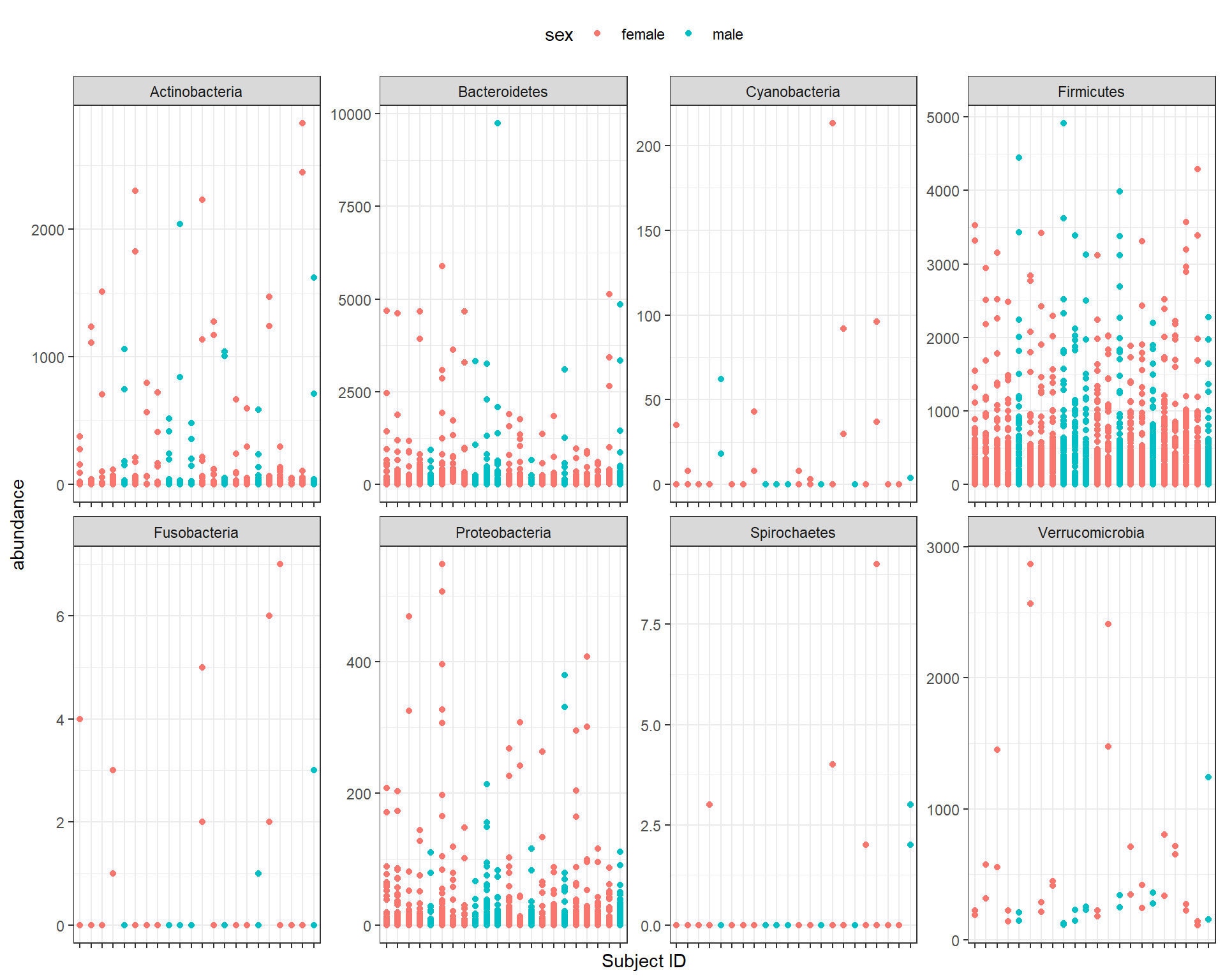

We can group the data by phylum and group and then use the nest function from the tidyr package to create a new dataframe containing the nested data:

library(tidyr)
nested_data <- peerj32_tibble %>%
  group_by(phylum, group) %>%
  nest()

slice(nested_data, 1:3)

## # A tibble: 16 × 3
## # Groups:   phylum, group [16]
##    group   phylum          data                
##    <fct>   <chr>           <list>              
##  1 LGG     Actinobacteria  <tibble [128 × 8]>  
##  2 Placebo Actinobacteria  <tibble [224 × 8]>  
##  3 LGG     Bacteroidetes   <tibble [256 × 8]>  
##  4 Placebo Bacteroidetes   <tibble [448 × 8]>  
##  5 LGG     Cyanobacteria   <tibble [16 × 8]>   
##  6 Placebo Cyanobacteria   <tibble [28 × 8]>   
##  7 LGG     Firmicutes      <tibble [1,216 × 8]>
##  8 Placebo Firmicutes      <tibble [2,128 × 8]>
##  9 LGG     Fusobacteria    <tibble [16 × 8]>   
## 10 Placebo Fusobacteria    <tibble [28 × 8]>   
## 11 LGG     Proteobacteria  <tibble [416 × 8]>  
## 12 Placebo Proteobacteria  <tibble [728 × 8]>  
## 13 LGG     Spirochaetes    <tibble [16 × 8]>   
## 14 Placebo Spirochaetes    <tibble [28 × 8]>   
## 15 LGG     Verrucomicrobia <tibble [16 × 8]>   
## 16 Placebo Verrucomicrobia <tibble [28 × 8]>

We can then use the map function from the purrr package to apply functions to each nested dataframe. Let’s start by counting the rows in each nested dataframe and filtering out dataframes with less than 25 rows.

library(purrr)

filtered_data <- nested_data %>%
  mutate(n_rows = purrr::map(data, ~ nrow(.x))) %>%
  filter(n_rows > 25)

Now let’s perform a t-test on each out the nested dataframes. Remember, each nested dataframe is one unique combination of phylum and group.

t_tests <- filtered_data %>%
  mutate(t_test = purrr::map(data, ~t.test(abundance ~ sex, data = .x)))

t_tests

## # A tibble: 12 × 5
## # Groups:   phylum, group [12]
##    group   phylum          data                 n_rows    t_test 
##    <fct>   <chr>           <list>               <list>    <list> 
##  1 LGG     Bacteroidetes   <tibble [256 × 8]>   <int [1]> <htest>
##  2 Placebo Bacteroidetes   <tibble [448 × 8]>   <int [1]> <htest>
##  3 Placebo Firmicutes      <tibble [2,128 × 8]> <int [1]> <htest>
##  4 LGG     Firmicutes      <tibble [1,216 × 8]> <int [1]> <htest>
##  5 Placebo Verrucomicrobia <tibble [28 × 8]>    <int [1]> <htest>
##  6 LGG     Actinobacteria  <tibble [128 × 8]>   <int [1]> <htest>
##  7 Placebo Actinobacteria  <tibble [224 × 8]>   <int [1]> <htest>
##  8 Placebo Proteobacteria  <tibble [728 × 8]>   <int [1]> <htest>
##  9 LGG     Proteobacteria  <tibble [416 × 8]>   <int [1]> <htest>
## 10 Placebo Cyanobacteria   <tibble [28 × 8]>    <int [1]> <htest>
## 11 Placebo Fusobacteria    <tibble [28 × 8]>    <int [1]> <htest>
## 12 Placebo Spirochaetes    <tibble [28 × 8]>    <int [1]> <htest>

The resulting dataframe contains a new column, which contains the model objects. Just as we mapped the t.test function, we can map the tidying functions from the broom package to extract the information we want from the nested model objects.

summary <- t_tests %>%
  mutate(summary = purrr::map(t_test, broom::glance))

summary

## # A tibble: 12 × 6
## # Groups:   phylum, group [12]
##    group   phylum          data                 n_rows    t_test  summary 
##    <fct>   <chr>           <list>               <list>    <list>  <list>  
##  1 LGG     Bacteroidetes   <tibble [256 × 8]>   <int [1]> <htest> <tibble>
##  2 Placebo Bacteroidetes   <tibble [448 × 8]>   <int [1]> <htest> <tibble>
##  3 Placebo Firmicutes      <tibble [2,128 × 8]> <int [1]> <htest> <tibble>
##  4 LGG     Firmicutes      <tibble [1,216 × 8]> <int [1]> <htest> <tibble>
##  5 Placebo Verrucomicrobia <tibble [28 × 8]>    <int [1]> <htest> <tibble>
##  6 LGG     Actinobacteria  <tibble [128 × 8]>   <int [1]> <htest> <tibble>
##  7 Placebo Actinobacteria  <tibble [224 × 8]>   <int [1]> <htest> <tibble>
##  8 Placebo Proteobacteria  <tibble [728 × 8]>   <int [1]> <htest> <tibble>
##  9 LGG     Proteobacteria  <tibble [416 × 8]>   <int [1]> <htest> <tibble>
## 10 Placebo Cyanobacteria   <tibble [28 × 8]>    <int [1]> <htest> <tibble>
## 11 Placebo Fusobacteria    <tibble [28 × 8]>    <int [1]> <htest> <tibble>
## 12 Placebo Spirochaetes    <tibble [28 × 8]>    <int [1]> <htest> <tibble>

The final step is to return a tidy dataframe, we can do this using the unnest function from the tidyr package. Note: it is also wise to ungroup after you are done operating on your grouped variables - you may run into problems if you forget your dataframe is grouped later on!

unnested <- summary %>%
  unnest(summary) %>%
  ungroup() %>%
  dplyr::select(group, phylum, p.value)

unnested

## # A tibble: 12 × 3
##    group   phylum          p.value
##    <fct>   <chr>             <dbl>
##  1 LGG     Bacteroidetes    0.930 
##  2 Placebo Bacteroidetes    0.828 
##  3 Placebo Firmicutes       0.344 
##  4 LGG     Firmicutes       0.131 
##  5 Placebo Verrucomicrobia  0.106 
##  6 LGG     Actinobacteria   0.600 
##  7 Placebo Actinobacteria   0.997 
##  8 Placebo Proteobacteria   0.856 
##  9 LGG     Proteobacteria   0.0111
## 10 Placebo Cyanobacteria    0.193 
## 11 Placebo Fusobacteria     0.265 
## 12 Placebo Spirochaetes     0.728

We can then plot the results. Let’s do this for the “LGG” (non-placebo) group, using our principles for good graphics.

p_data <- unnested %>%
  filter(group == "LGG") %>%
  mutate(phylum = fct_reorder(phylum, p.value))
  
ggplot(p_data, aes(y = p.value, x = phylum)) +
  facet_wrap(~group) +
  geom_bar(stat="identity", fill = "grey90", color = "grey20") +
  coord_flip() +
  theme_bw() +
  ggtitle("Difference in abundance by gender") +
  xlab("") + ylab("p-value from t-test")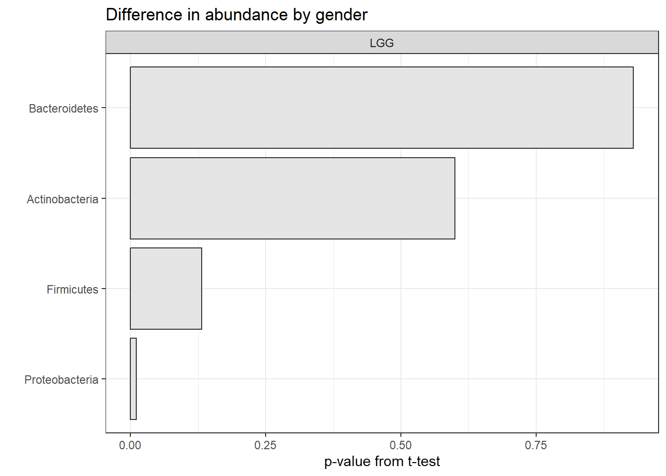

7.5 Regression models

Download a pdf of the lecture slides for this video.

7.5.1 Formula structure

Regression models can be used to estimate how the expected value of a dependent variable changes as independent variables change.

In R, regression formulas take this structure:

## Generic code
[response variable] ~ [indep. var. 1] +  [indep. var. 2] + ...

Notice that a tilde, ~, is used to separate the independent and dependent variables and that a plus sign, +, is used to join independent variables. This format mimics the statistical notation:

\[ Y_i \sim X_1 + X_2 + X_3 \]

You will use this type of structure in R fo a lot of different function calls, including those for linear models (fit with the lm function) and generalized linear models (fit with the glm function).

There are some conventions that can be used in R formulas. Common ones include:

Convention	Meaning
`I()`	evaluate the formula inside `I()` before fitting (e.g., `I(x1 + x2)`)
`:`	fit the interaction between `x1` and `x2` variables
`*`	fit the main effects and interaction for both variables (e.g., `x1*x2` equals `x1 + x2 + x1:x2`)
`.`	include as independent variables all variables other than the response (e.g., `y ~ .`)
`1`	intercept (e.g., `y ~ 1` for an intercept-only model)
`-`	do not include a variable in the data frame as an independent variables (e.g., `y ~ . - x1`); usually used in conjunction with `.` or `1`

7.5.2 Linear models

To fit a linear model, you can use the function lm(). This function is part of the stats package, which comes installed with base R. In this function, you can use the data option to specify the data frame from which to get the vectors.

## Warning: There was 1 warning in `mutate()`.
## ℹ In argument: `sex = fct_recode(factor(sex), Male = "1", Female = "2")`.
## Caused by warning:
## ! Unknown levels in `f`: 1, 2

mod_a <- lm(wt ~ ht, data = nepali)

This previous call fits the model:

\[ Y_{i} = \beta_{0} + \beta_{1}X_{1,i} + \epsilon_{i} \]

where:

$Y_{i}$ : weight of child $i$
$X_{1,i}$ : height of child $i$

If you run the lm function without saving it as an object, R will fit the regression and print out the function call and the estimated model coefficients:

lm(wt ~ ht, data = nepali)

## 
## Call:
## lm(formula = wt ~ ht, data = nepali)
## 
## Coefficients:
## (Intercept)           ht  
##     -8.7581       0.2342

However, to be able to use the model later for things like predictions and model assessments, you should save the output of the function as an R object:

mod_a <- lm(wt ~ ht, data = nepali)

This object has a special class, lm:

class(mod_a)

## [1] "lm"

This class is a special type of list object. If you use is.list to check, you can confirm that this object is a list:

is.list(mod_a)

## [1] TRUE

There are a number of functions that you can apply to an lm object. These include:

Function	Description
`summary`	Get a variety of information on the model, including coefficients and p-values for the coefficients
`coefficients`	Pull out just the coefficients for a model
`fitted`	Get the fitted values from the model (for the data used to fit the model)
`plot`	Create plots to help assess model assumptions
`residuals`	Get the model residuals

For example, you can get the coefficients from the model by running:

coefficients(mod_a)

## (Intercept)          ht 
##  -8.7581466   0.2341969

The estimated coefficient for the intercept is always given under the name “(Intercept)”. Estimated coefficients for independent variables are given based on their column names in the original data (“ht” here, for $\beta_1$, or the estimated increase in expected weight for a one unit increase in height).

You can use the output from a coefficients call to plot a regression line based on the model fit on top of points showing the original data (Figure 7.1).

mod_coef <- coefficients(mod_a)
ggplot(nepali, aes(x = ht, y = wt)) + 
  geom_point(size = 0.2) + 
  xlab("Height (cm)") + ylab("Weight (kg)") + 
  geom_abline(aes(intercept = mod_coef[1],
                  slope = mod_coef[2]), col = "blue")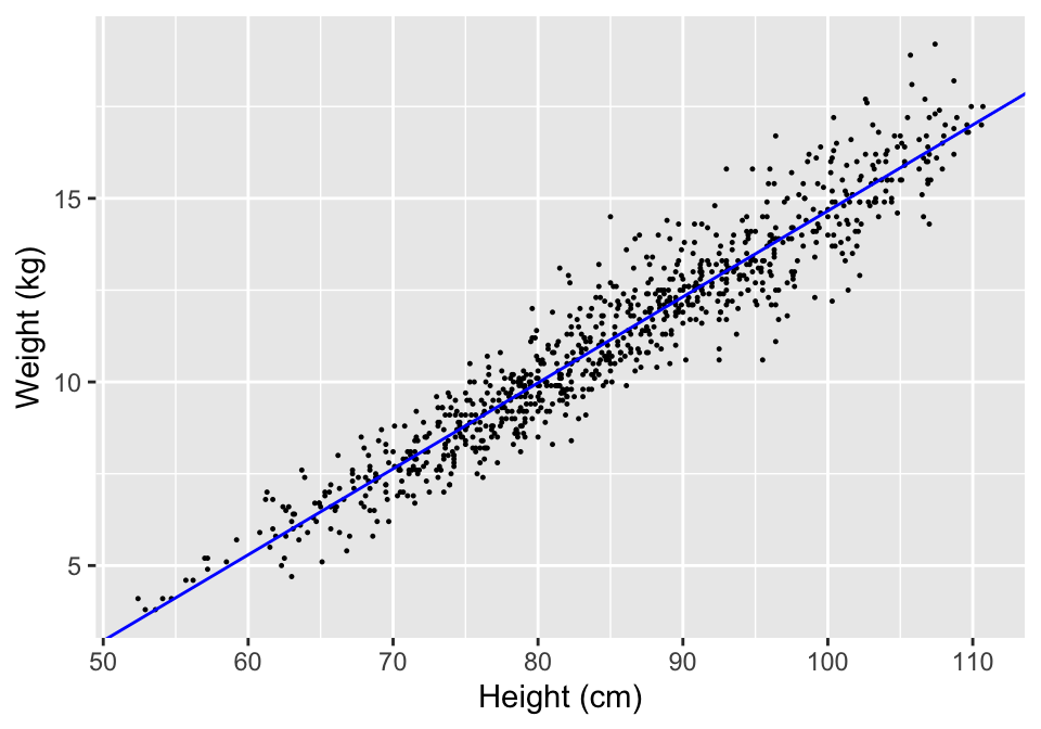

Figure 7.1: Example of using the output from a coefficients call to add a regression line to a scatterplot.

You can also add a linear regression line to a scatterplot by adding the geom geom_smooth using the argument method = “lm”.

You can use the function residuals on an lm object to pull out the residuals from the model fit:

head(residuals(mod_a))

##          1          2          3          4          6          7 
##  0.1993922 -0.4329393 -0.4373953 -0.1355300 -0.6749080 -1.0838199

The result of a residuals call is a vector with one element for each of the non-missing observations (rows) in the data frame you used to fit the model. Each value gives the different between the model fitted value and the observed value for each of these observations, in the same order the observations show up in the data frame. The residuals are in the same order as the observations in the original data frame.

You can also use the shorter function coef as an alternative to coefficients and the shorter function resid as an alternative to residuals.

As noted in the subsection on simple statistics functions, the summary function returns different output depending on the type of object that is input to the function. If you input a regression model object to summary, the function gives you a lot of information about the model. For example, here is the output returned by running summary for the linear regression model object we just created:

summary(mod_a)

## 
## Call:
## lm(formula = wt ~ ht, data = nepali)
## 
## Residuals:
##     Min      1Q  Median      3Q     Max 
## -3.0077 -0.5479 -0.0293  0.4972  3.3514 
## 
## Coefficients:
##              Estimate Std. Error t value Pr(>|t|)    
## (Intercept) -8.758147   0.211529  -41.40   <2e-16 ***
## ht           0.234197   0.002459   95.23   <2e-16 ***
## ---
## Signif. codes:  0 '***' 0.001 '**' 0.01 '*' 0.05 '.' 0.1 ' ' 1
## 
## Residual standard error: 0.8733 on 875 degrees of freedom
##   (123 observations deleted due to missingness)
## Multiple R-squared:  0.912,  Adjusted R-squared:  0.9119 
## F-statistic:  9068 on 1 and 875 DF,  p-value: < 2.2e-16

This output includes a lot of useful elements, including (1) basic summary statistics for the residuals (to meet model assumptions, the median should be around zero and the absolute values fairly similar for the first and third quantiles), (2) coefficient estimates, standard errors, and p-values, and (3) some model summary statistics, including residual standard error, degrees of freedom, number of missing observations, and F-statistic.

The object returned by the summary() function when it is applied to an lm object is a list, which you can confirm using the is.list function:

is.list(summary(mod_a))

## [1] TRUE

With any list, you can use the names function to get the names of all of the different elements of the object:

names(summary(mod_a))

##  [1] "call"          "terms"         "residuals"     "coefficients" 
##  [5] "aliased"       "sigma"         "df"            "r.squared"    
##  [9] "adj.r.squared" "fstatistic"    "cov.unscaled"  "na.action"

You can use the $ operator to pull out any element of the list. For example, to pull out the table with information on the estimated model coefficients, you can run:

summary(mod_a)$coefficients

##               Estimate  Std. Error   t value      Pr(>|t|)
## (Intercept) -8.7581466 0.211529182 -41.40396 2.411051e-208
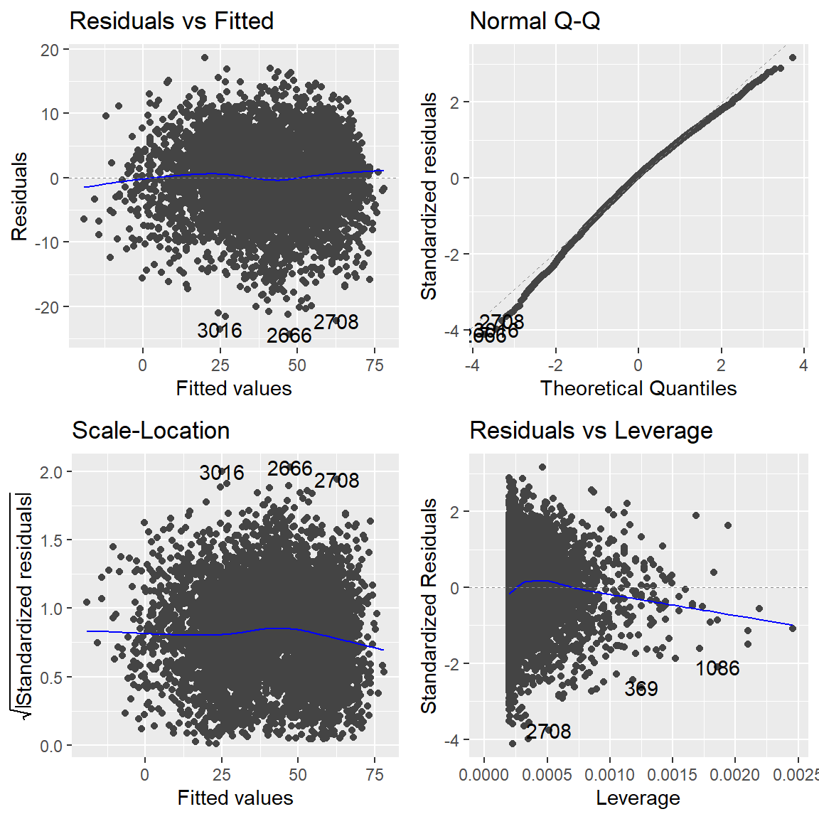
## ht           0.2341969 0.002459347  95.22726  0.000000e+00

The plot function, like the summary function, will give different output depending on the class of the object that you input. For an lm object, you can use the plot function to get a number of useful diagnostic plots that will help you check regression assumptions (Figure 7.2):

plot(mod_a)

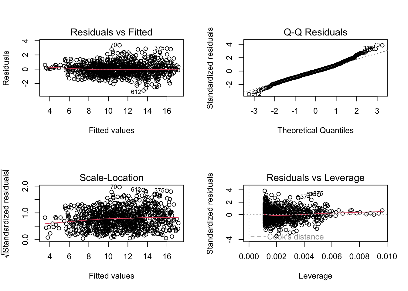
Figure 7.2: Example output from running the plot function with an lm object as the input.

You can also use binary variables or factors as independent variables in regression models. For example, in the nepali dataset, sex is a factor variable with the levels “Male” and “Female”. You can fit a linear model of weight regressed on sex for this data with the call:

mod_b <- lm(wt ~ sex, data = nepali)

This call fits the model:

\[ Y_{i} = \beta_{0} + \beta_{1}X_{1,i} + \epsilon_{i} \]

where $X_{1,i}$ : sex of child $i$, where 0 = male and 1 = female.

Here are the estimated coefficients from fitting this model:

summary(mod_b)$coefficients

##               Estimate Std. Error   t value   Pr(>|t|)
## (Intercept) 11.4226374  0.1375427 83.047920 0.00000000
## sexFemale   -0.4866184  0.1982810 -2.454185 0.01431429

You’ll notice that, in addition to an estimated intercept ((Intercept)), the other estimated coefficient is sexFemale rather than just sex, although the column name in the data frame input to lm for this variable is sex.

This is because, when a factor or binary variable is input as an independent variable in a linear regression model, R will fit an estimated coefficient for all levels of factors except the first factor level. By default, this first factor level is used as the baseline level, and so its estimated mean is given by the estimated intercept, while the other model coefficients give the estimated difference from this baseline.

For example, the model fit above tells us that the estimated mean weight of males is 11.4, while the estimated mean weight of females is 11.4 + -0.5 = 10.9.

7.6 Handling model objects

The broom package contains tools for converting statistical objects into nice tidy data frames. The tools in the broom package make it easy to process statistical results in R using the tools of the tidyverse.

7.6.1 broom::tidy

The tidy() function returns a data frame with information on the fitted model terms. For example, when applied to one of our linear models we get:

  library(broom)
  kable(tidy(mod_a), digits = 3)

term	estimate	std.error	statistic	p.value
(Intercept)	-8.758	0.212	-41.404	0
ht	0.234	0.002	95.227	0

  class(tidy(mod_a))

## [1] "tbl_df"     "tbl"        "data.frame"

You can pass arguments to the tidy() function. For example, include confidence intervals:

  kable(tidy(mod_a, conf.int = TRUE), digits = 3)

term	estimate	std.error	statistic	p.value	conf.low	conf.high
(Intercept)	-8.758	0.212	-41.404	0	-9.173	-8.343
ht	0.234	0.002	95.227	0	0.229	0.239

7.6.2 broom::augment

The augment() function adds information about a fitted model to the dataset used to fit the model. For example, when applied to one of our linear models we get information on the fitted values and residuals included in the output:

  kable(head(broom::augment(mod_a), 3), digits = 3)

.rownames	wt	ht	.fitted	.resid	.hat	.sigma	.std.resid
1	12.8	91.2	12.601	0.199	0.001	0.874	0.228
2	12.8	93.9	13.233	-0.433	0.002	0.874	-0.496
3	13.1	95.2	13.537	-0.437	0.002	0.874	-0.501

7.6.3 broom::glance

The glance() functions returns a one row summary of a fitted model object: For example:

  kable(glance(mod_a, conf.int = TRUE), digits = 3)

r.squared	adj.r.squared	sigma	statistic	p.value	df	logLik	AIC	BIC	deviance	df.residual	nobs
0.912	0.912	0.873	9068.23	0	1	-1124.615	2255.23	2269.56	667.351	875	877

7.6.4 References– statistics in R

One great (and free online for CSU students through our library) book to find out more about using R for basic statistics is:

Introductory Statistics with R

If you want all the details about fitting linear models and GLMs in R, Julian Faraway’s books are fantastic. He has one on linear models and one on extensions including logistic and Poisson models:

Linear Models with R (also free online through the CSU library)
Extending the Linear Model with R

7.7 Functions

Download a pdf of the lecture slides for this video.

As you move to larger projects, you will find yourself using the same code a lot.

Examples include:

Reading in data from a specific type of equipment (air pollution monitor, accelerometer)
Running a specific type of analysis
Creating a specific type of plot or map

If you find yourself cutting and pasting a lot, convert the code to a function.

Advantages of writing functions include:

Coding is more efficient
Easier to change your code (if you’ve cut and paste code and you want to change something, you have to change it everywhere - this is an easy way to accidentally create bugs in your code)
Easier to share code with others

You can name a function anything you want (although try to avoid names of preexisting-existing functions). You then define any inputs (arguments; separate multiple arguments with commas) and put the code to run in braces:

## Note: this code will not run
[function name] <- function([any arguments]){
        [code to run]
}

Here is an example of a very basic function. This function takes a number as input and adds 1 to that number.

add_one <- function(number){
  out <- number + 1
  return(out)
}

add_one(number = 3)

## [1] 4

add_one(number = -1)

## [1] 0

Functions can input any type of R object (for example, vectors, data frames, even other functions and ggplot objects)
Similarly, functions can output any type of R object
When defining a function, you can set default values for some of the parameters
You can explicitly specify the value to return from the function

For example, the following function inputs a data frame (datafr) and a one-element vector (child_id) and returns only rows in the data frame where it’s id column matches child_id. It includes a default value for datafr, but not for child_id.

subset_nepali <- function(datafr = nepali, child_id){
  datafr <- datafr %>%
            filter(id == child_id)
  return(datafr)
}

If an argument is not given for a parameter with a default, the function will run using the default value for that parameter. For example:

subset_nepali(child_id = "120011")

##       id  sex   wt   ht mage lit died alive age
## 1 120011 Male 12.8 91.2   35   0    2     5  41
## 2 120011 Male 12.8 93.9   35   0    2     5  45
## 3 120011 Male 13.1 95.2   35   0    2     5  49
## 4 120011 Male 13.8 96.9   35   0    2     5  53
## 5 120011 Male   NA   NA   35   0    2     5  57

If an argument is not given for a parameter without a default, the function call will result in an error. For example:

subset_nepali(datafr = nepali)

## Error in `filter()`:
## ℹ In argument: `id == child_id`.
## Caused by error:
## ! argument "child_id" is missing, with no default

By default, the function will return the last defined object, although the choice of using return can affect printing behavior when you run the function. For example, I could have written the subset_nepali function like this:

subset_nepali <- function(datafr = nepali, child_id){
  datafr <- datafr %>%
            filter(id == child_id)
}

In this case, the output will not automatically print out when you call the function without assigning it to an R object:

subset_nepali(child_id = "120011")

However, the output can be assigned to an R object in the same way as when the function was defined without return:

first_childs_data <- subset_nepali(child_id = "120011")
first_childs_data

##       id  sex   wt   ht mage lit died alive age
## 1 120011 Male 12.8 91.2   35   0    2     5  41
## 2 120011 Male 12.8 93.9   35   0    2     5  45
## 3 120011 Male 13.1 95.2   35   0    2     5  49
## 4 120011 Male 13.8 96.9   35   0    2     5  53
## 5 120011 Male   NA   NA   35   0    2     5  57

R is very “good” at running functions! It will look for (scope) the variables in your function in various places (environments). So your functions may run even when you don’t expect them to, potentially, with unexpected results!

The return function can also be used to return an object other than the last defined object (although this doesn’t tend to be something you need to do very often). If you did not use return in the following code, it will output “Test output”:

subset_nepali <- function(datafr = nepali, child_id){
  datafr <- datafr %>%
            filter(id == child_id)
  a <- "Test output"
}
(subset_nepali(child_id = "120011"))

## [1] "Test output"

Conversely, you can use return to output datafr, even though it’s not the last object defined:

subset_nepali <- function(datafr = nepali, child_id){
  datafr <- datafr %>%
            filter(id == child_id)
  a <- "Test output"
  return(datafr)
}
subset_nepali(child_id = "120011")

##       id  sex   wt   ht mage lit died alive age
## 1 120011 Male 12.8 91.2   35   0    2     5  41
## 2 120011 Male 12.8 93.9   35   0    2     5  45
## 3 120011 Male 13.1 95.2   35   0    2     5  49
## 4 120011 Male 13.8 96.9   35   0    2     5  53
## 5 120011 Male   NA   NA   35   0    2     5  57

7.7.1 if / else statements

There are other control structures you can use in your R code. Two that you will commonly use within R functions are if and ifelse statements.

An if statement tells R that, if a certain condition is true, do run some code. For example, if you wanted to print out only odd numbers between 1 and 5, one way to do that is with an if statement: (Note: the %% operator in R returns the remainder of the first value (i) divided by the second value (2).)

for(i in 1:5){
  if(i %% 2 == 1){
    print(i)
  }
}

## [1] 1
## [1] 3
## [1] 5

The if statement runs some code if a condition is true, but does nothing if it is false. If you’d like different code to run depending on whether the condition is true or false, you can us an if / else or an if / else if / else statement.

for(i in 1:5){
  if(i %% 2 == 1){
    print(i)
  } else {
    print(paste(i, "is even"))
  }
}

## [1] 1
## [1] "2 is even"
## [1] 3
## [1] "4 is even"
## [1] 5

What would this code do?

for(i in 1:100){
  if(i %% 3 == 0 & i %% 5 == 0){
    print("FizzBuzz")
  } else if(i %% 3 == 0){
    print("Fizz")
  } else if(i %% 5 == 0){
    print("Buzz")
  } else {
    print(i)
  }
}

If / else statements are extremely useful in functions.

In R, the if statement evaluates everything in the parentheses and, if that evaluates to TRUE, runs everything in the braces. This means that you can trigger code in an if statement with a single-value logical vector:

weekend <- TRUE
if(weekend){
  print("It's the weekend!")
}

## [1] "It's the weekend!"

This functionality can be useful with parameters you choose to include when writing your own functions (e.g., print = TRUE).

7.7.2 Some other control structures

The control structure you are most likely to use in data analysis with R is the “if / else” statement. However, there are a few other control structures you may occasionally find useful:

next
break
while

You can use the next structure to skip to the next round of a loop when a certain condition is met. For example, we could have used this code to print out odd numbers between 1 and 5:

i <- 0
while(i < 5){
  i <- 1 + i
  if(i %% 2 == 0){
    next
  }
  print(i)
}

## [1] 1
## [1] 3
## [1] 5

You can use break to break out of a loop if a certain condition is met. For example, the final code will break out of the loop once i is over 2, so it will only print the numbers 1 through 3:

i <- 0
while(i <= 5){
  if(i > 2){
    break
  }
  i <- 1 + i
  print(i)
}

## [1] 1
## [1] 2
## [1] 3

7.8 In-course exercise for Chapter 7

7.8.1 Exploring taxonomic profiling data

We’ll be using a package on Bioconductor called microbiome. You’ll need to install that package from Bioconductor. This uses code that’s different from the default you use to download a package from CRAN. Go to the Bioconductor page for the microbiome package and figure out how to install this package based on instructions on that page.
The microbiome that includes tools for exploring and analysing microbiome profiling data. This package has a website with tutorial information here. We want to explore a dataset on genus-level microbiota profiling (atlas1006). Navigate to the tutorial webpage to figure out how you can get this example raw data loaded in your R session. Use the class and str functions to start exploring this data. Is it in a dataframe (tibble)? Is it in a tidy format? How is the data structured?
On the microbiome page, find the documentation describing the atlas1006 data. Look through this documentation to figure out what information is included in the data. Also, check the helpfile for this dataset and look up the original article describing the data (you can find the article information in the help resources).
The atlas1006 data is stored in a special object class called a “phyloseq” object (you should have seen this when you used class with the object). You can pull certain parts of this data using special functions called “accessors”. One is get_variable. Try running get_variable with the atlas1006 data. What do you think this data is showing?
Which different nationalities are represented by the study subjects, based on the dataframe you extracted in the last step? How many samples have each nationality? Which different BMI groups are included? Does it look like the study was balanced among these groups?
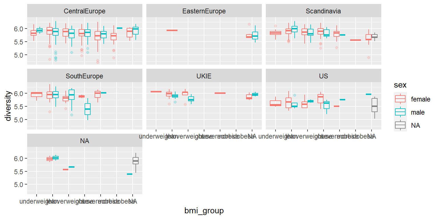
Based on the data you extracted, does it look like diversity varies much between males and females? Across BMI groups?
Discuss what steps you would need to take to create the following plot. To start, don’t write any code, just develop a plan. Talk about what the dataset should look like right before you create the plot and what functions you could use to get the data from its current format to that format.
Try to write the code to create this plot. This will include some code for cleaning the data and some code for plotting. I will add one example answer after class, but I’d like you to try to figure it out yourselves first.

7.8.1.1 Example R code

Install the microbiome package from Bioconductor:

if (!requireNamespace("BiocManager", quietly = TRUE))
    install.packages("BiocManager")

BiocManager::install("microbiome")

Load the atlas1006 example data in the microbiome package and explore it with str and class:

library(microbiome)
data(atlas1006)

class(atlas1006)

## [1] "phyloseq"
## attr(,"package")
## [1] "phyloseq"

str(atlas1006)

## Formal class 'phyloseq' [package "phyloseq"] with 5 slots
##   ..@ otu_table:Formal class 'otu_table' [package "phyloseq"] with 2 slots
##   .. .. ..@ .Data        : num [1:130, 1:1151] 0 0 0 21 1 72 0 0 176 10 ...
##   .. .. .. ..- attr(*, "dimnames")=List of 2
##   .. .. .. .. ..$ : chr [1:130] "Actinomycetaceae" "Aerococcus" "Aeromonas" "Akkermansia" ...
##   .. .. .. .. ..$ : chr [1:1151] "Sample-1" "Sample-2" "Sample-3" "Sample-4" ...
##   .. .. ..@ taxa_are_rows: logi TRUE
##   .. .. ..$ dim     : int [1:2] 130 1151
##   .. .. ..$ dimnames:List of 2
##   .. .. .. ..$ : chr [1:130] "Actinomycetaceae" "Aerococcus" "Aeromonas" "Akkermansia" ...
##   .. .. .. ..$ : chr [1:1151] "Sample-1" "Sample-2" "Sample-3" "Sample-4" ...
##   ..@ tax_table:Formal class 'taxonomyTable' [package "phyloseq"] with 1 slot
##   .. .. ..@ .Data: chr [1:130, 1:3] "Actinobacteria" "Firmicutes" "Proteobacteria" "Verrucomicrobia" ...
##   .. .. .. ..- attr(*, "dimnames")=List of 2
##   .. .. .. .. ..$ : chr [1:130] "Actinomycetaceae" "Aerococcus" "Aeromonas" "Akkermansia" ...
##   .. .. .. .. ..$ : chr [1:3] "Phylum" "Family" "Genus"
##   .. .. ..$ dim     : int [1:2] 130 3
##   .. .. ..$ dimnames:List of 2
##   .. .. .. ..$ : chr [1:130] "Actinomycetaceae" "Aerococcus" "Aeromonas" "Akkermansia" ...
##   .. .. .. ..$ : chr [1:3] "Phylum" "Family" "Genus"
##   ..@ sam_data :'data.frame':    1151 obs. of  10 variables:
## Formal class 'sample_data' [package "phyloseq"] with 4 slots
##   .. .. ..@ .Data    :List of 10
##   .. .. .. ..$ : int [1:1151] 28 24 52 22 25 42 25 27 21 25 ...
##   .. .. .. ..$ : Factor w/ 2 levels "female","male": 2 1 2 1 1 2 1 1 1 1 ...
##   .. .. .. ..$ : Factor w/ 6 levels "CentralEurope",..: 6 6 6 6 6 6 6 6 6 6 ...
##   .. .. .. ..$ : Factor w/ 3 levels "o","p","r": NA NA NA NA NA NA NA NA NA NA ...
##   .. .. .. ..$ : Factor w/ 40 levels "1","2","3","4",..: 1 1 1 1 1 1 1 1 1 1 ...
##   .. .. .. ..$ : num [1:1151] 5.76 6.06 5.5 5.87 5.89 5.53 5.49 5.38 5.34 5.64 ...
##   .. .. .. ..$ : Factor w/ 6 levels "underweight",..: 5 4 2 1 2 2 1 2 2 2 ...
##   .. .. .. ..$ : Factor w/ 1006 levels "1","2","3","4",..: 1 2 3 4 5 6 7 8 9 10 ...
##   .. .. .. ..$ : num [1:1151] 0 0 0 0 0 0 0 0 0 0 ...
##   .. .. .. ..$ : chr [1:1151] "Sample-1" "Sample-2" "Sample-3" "Sample-4" ...
##   .. .. ..@ names    : chr [1:10] "age" "sex" "nationality" "DNA_extraction_method" ...
##   .. .. ..@ row.names: chr [1:1151] "Sample-1" "Sample-2" "Sample-3" "Sample-4" ...
##   .. .. ..@ .S3Class : chr "data.frame"
##   ..@ phy_tree : NULL
##   ..@ refseq   : NULL

Pull out the data frame that contains information on each study subject in the atlas1006 data by using the get_variable accessor function:

get_variable(atlas1006) %>% head()

##          age    sex nationality DNA_extraction_method project diversity
## Sample-1  28   male          US                  <NA>       1      5.76
## Sample-2  24 female          US                  <NA>       1      6.06
## Sample-3  52   male          US                  <NA>       1      5.50
## Sample-4  22 female          US                  <NA>       1      5.87
## Sample-5  25 female          US                  <NA>       1      5.89
## Sample-6  42   male          US                  <NA>       1      5.53
##            bmi_group subject time   sample
## Sample-1 severeobese       1    0 Sample-1
## Sample-2       obese       2    0 Sample-2
## Sample-3        lean       3    0 Sample-3
## Sample-4 underweight       4    0 Sample-4
## Sample-5        lean       5    0 Sample-5
## Sample-6        lean       6    0 Sample-6

Note: Since the first argument to get_variable is the phyloseq object (here, the atlas1006 data object), you can pipe into the function, like this:

atlas1006 %>% 
  get_variable() %>% 
  head()

Find out the different nationalities included in the data:

atlas1006 %>% 
  get_variable() %>% 
  as_tibble() %>% # Change output from a data.frame to a tibble
  group_by(nationality) %>% 
  count()

## # A tibble: 7 × 2
## # Groups:   nationality [7]
##   nationality       n
##   <fct>         <int>
## 1 CentralEurope   650
## 2 EasternEurope    15
## 3 Scandinavia     271
## 4 SouthEurope      89
## 5 UKIE             50
## 6 US               44
## 7 <NA>             32

It looks like most subjects were from Central Europe, with the next-largest group from Scandinavia. Note: If you wanted to rearrange this summary to give the nationalities in order of the number of subjects in each, you could add on a forcats function:

atlas1006 %>% 
  get_variable() %>% 
  as_tibble() %>% # Change output from a data.frame to a tibble
  mutate(nationality = fct_infreq(nationality)) %>% 
  group_by(nationality) %>% 
  count()

## # A tibble: 7 × 2
## # Groups:   nationality [7]
##   nationality       n
##   <fct>         <int>
## 1 CentralEurope   650
## 2 Scandinavia     271
## 3 SouthEurope      89
## 4 UKIE             50
## 5 US               44
## 6 EasternEurope    15
## 7 <NA>             32

Find out the different BMI groups included in the data and if the study seemed to be balanced across those groups:

atlas1006 %>% 
  get_variable() %>% 
  as_tibble() %>% # Change output from a data.frame to a tibble
  group_by(bmi_group) %>% 
  count()

## # A tibble: 7 × 2
## # Groups:   bmi_group [7]
##   bmi_group       n
##   <fct>       <int>
## 1 underweight    21
## 2 lean          484
## 3 overweight    197
## 4 obese         222
## 5 severeobese    99
## 6 morbidobese    22
## 7 <NA>          106

There were six different BMI groups. Over 100 study subjects had this information missing. The samples were not evenly distributed across these BMI groups. Instead, the most common (lean) had almost 500 subjects, while the smaller BMI-group samples were around 20 people.

See if it looks like diversity varies much between males and females:

atlas1006 %>% 
  get_variable() %>% 
  as_tibble() %>% 
  group_by(sex) %>% 
  summarize(mean_diversity = mean(diversity))

## # A tibble: 3 × 2
##   sex    mean_diversity
##   <fct>           <dbl>
## 1 female           5.84
## 2 male             5.85
## 3 <NA>             5.76

See if it looks like diversity varies much across BMI groups:

atlas1006 %>% 
  get_variable() %>% 
  as_tibble() %>% 
  group_by(bmi_group) %>% 
  summarize(mean_diversity = mean(diversity))

## # A tibble: 7 × 2
##   bmi_group   mean_diversity
##   <fct>                <dbl>
## 1 underweight           5.84
## 2 lean                  5.89
## 3 overweight            5.83
## 4 obese                 5.82
## 5 severeobese           5.74
## 6 morbidobese           5.67
## 7 <NA>                  5.81

Here is the code for the plot:

library(tidyverse)
library(ggthemes)
library(microbiome)

data(atlas1006)

atlas1006 %>% 
  get_variable() %>% 
  ggplot(aes(x = bmi_group, y = diversity, color = sex)) + 
  geom_boxplot(alpha = 0.2) + 
  facet_wrap(~ nationality)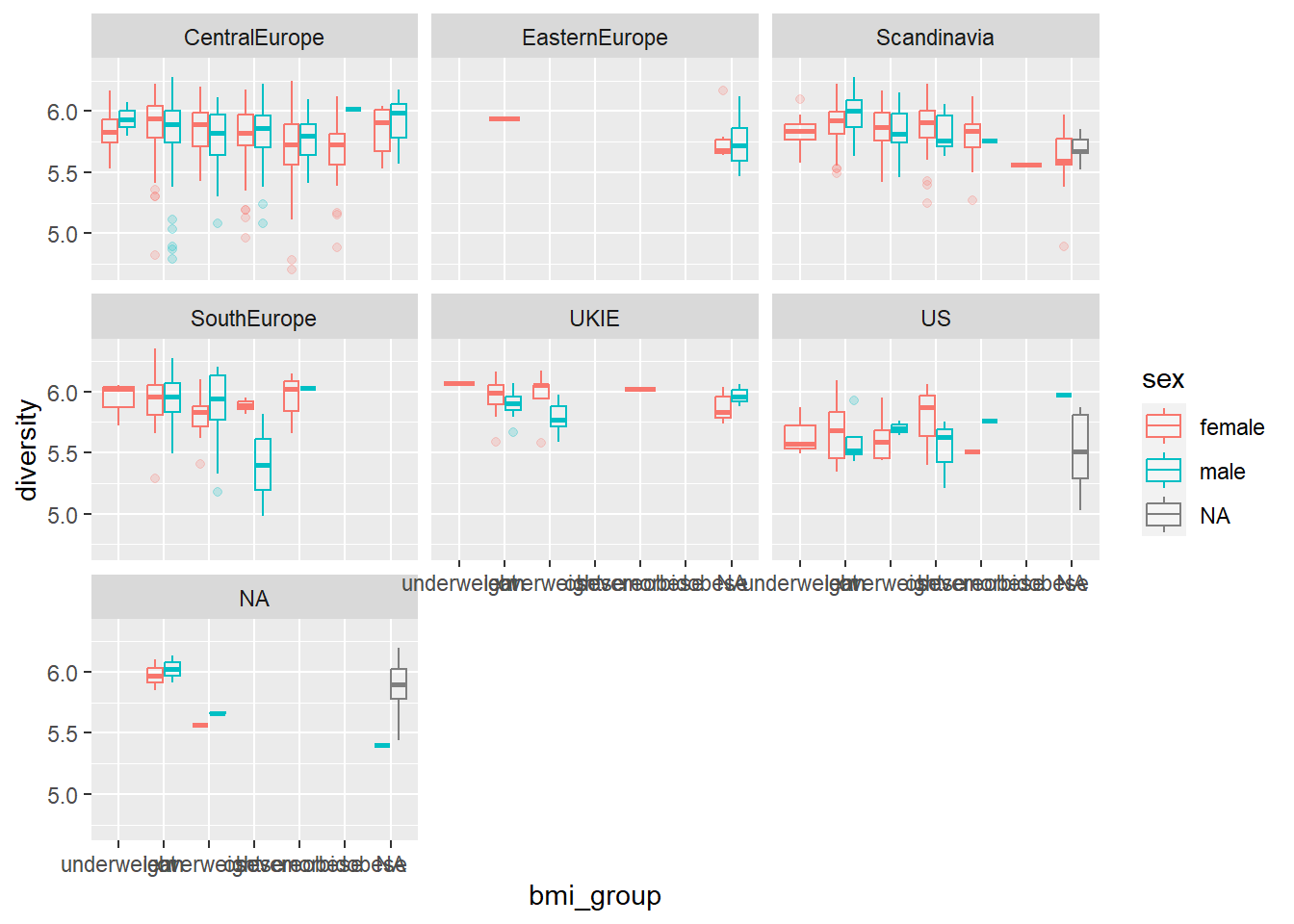

7.8.2 More with baby names

Let’s look at baby names that we started looking at last class, based on the letter they start with.

For the full dataframe, what proportion of baby names start with each letter? See if you can create a figure to help show this. Create the same plot using the names of people from our class.
What proportion of names start with “C” or “S” across the full dataset?

7.8.2.1 Example R code

For the full dataframe, what proportion of baby names start with “S”?

To start, create a column with the first letter of each name. You can use functions in the stringr package to do this. The easiest might be to use the position of the first letter to pull that information.

library(babynames)
library(stringr)
top_letters <- babynames %>% 
  mutate(first_letter = str_sub(name, 1, 1))

top_letters %>% 
  select(name, first_letter) %>% 
  slice(1:5)

## # A tibble: 5 × 2
##   name      first_letter
##   <chr>     <chr>       
## 1 Mary      M           
## 2 Anna      A           
## 3 Emma      E           
## 4 Elizabeth E           
## 5 Minnie    M

Now we can group by letter and figure out these proportions. First, while the data is grouped, count the number of names with each letter. Then, ungroup and use mutate to divide this by the total number of names:

top_letters <- top_letters %>% 
  group_by(first_letter) %>% 
  summarize(n = sum(n)) %>% 
  ungroup() %>% 
  mutate(prop = n / sum(n)) %>% 
  arrange(desc(prop))

top_letters

## # A tibble: 26 × 3
##    first_letter        n   prop
##    <chr>           <int>  <dbl>
##  1 J            44612175 0.128 
##  2 M            32864210 0.0944
##  3 A            28855232 0.0829
##  4 C            25533863 0.0733
##  5 D            24240271 0.0696
##  6 R            23702794 0.0681
##  7 S            21373830 0.0614
##  8 L            18942067 0.0544
##  9 E            17033760 0.0489
## 10 K            17006684 0.0489
## # ℹ 16 more rows

Here’s one way to visualize this:

library(scales)
top_letters %>% 
  mutate(first_letter = fct_reorder(first_letter, prop)) %>% 
  ggplot(aes(x = first_letter)) + 
  geom_bar(aes(weight = prop)) + 
  coord_flip() + 
  scale_y_continuous(labels = percent) + 
  labs(x = "", y = "Percent of names that start with ...")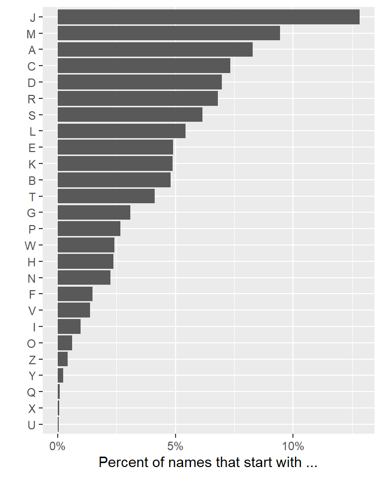

Create the same plot using the names of people in our class. First, create a vector with the names of people in our class:

student_list <- data_frame(name = c("Burton", "Caroline", "Chaoyu", "Collin",
                                    "Daniel", "Eric", "Erin", "Heather",
                                    "Jacob", "Jessica", "Khum", "Kyle",
                                    "Matthew", "Molly", "Nikki", "Rachel",
                                    "Sere",  "Shayna", "Sherry", "Sunny"))
student_list <- student_list %>% 
  mutate(first_letter = str_sub(name, 1, 1))
student_list

## # A tibble: 20 × 2
##    name     first_letter
##    <chr>    <chr>       
##  1 Burton   B           
##  2 Caroline C           
##  3 Chaoyu   C           
##  4 Collin   C           
##  5 Daniel   D           
##  6 Eric     E           
##  7 Erin     E           
##  8 Heather  H           
##  9 Jacob    J           
## 10 Jessica  J           
## 11 Khum     K           
## 12 Kyle     K           
## 13 Matthew  M           
## 14 Molly    M           
## 15 Nikki    N           
## 16 Rachel   R           
## 17 Sere     S           
## 18 Shayna   S           
## 19 Sherry   S           
## 20 Sunny    S

library(scales)
student_list %>% 
  group_by(first_letter) %>% 
  count() %>% 
  ungroup() %>% 
  mutate(prop = n / sum(n)) %>% 
  mutate(first_letter = fct_reorder(first_letter, prop)) %>% 
  ggplot(aes(x = first_letter)) + 
  geom_bar(aes(weight = prop)) + 
  coord_flip() + 
  scale_y_continuous(labels = percent) + 
  labs(x = "", y = "Percent of students with\na name that starts with ...")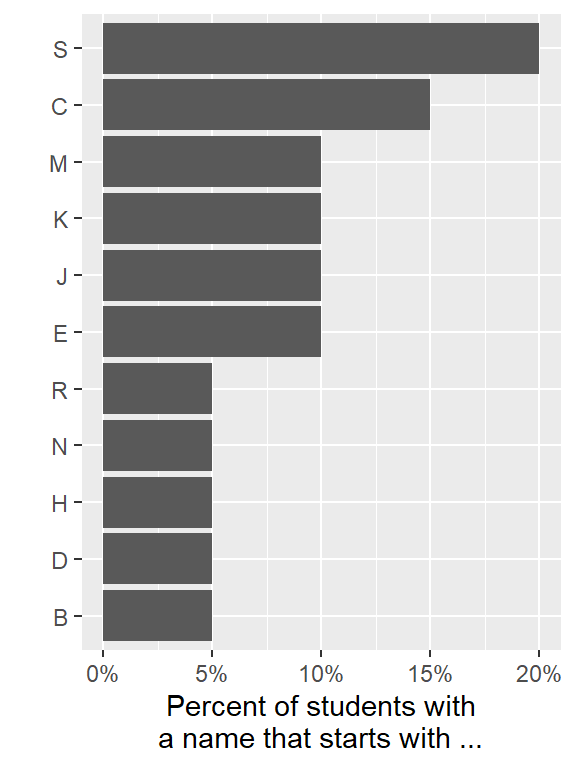

What proportion of names start with “C” or “S” across the full dataset? You can create a dataframe that (1) pulls out the first letter of each name (just like we did for the last part of the question) and (2) tests whether that first letter is an “A” or a “K” (using a logical statement):

c_or_s <- babynames %>% 
  mutate(first_letter = str_sub(name, 1, 1),
         c_or_s = first_letter %in% c("C", "S"))

c_or_s %>% 
  select(name, first_letter, c_or_s) %>% 
  slice(1:5)

## # A tibble: 5 × 3
##   name      first_letter c_or_s
##   <chr>     <chr>        <lgl> 
## 1 Mary      M            FALSE 
## 2 Anna      A            FALSE 
## 3 Emma      E            FALSE 
## 4 Elizabeth E            FALSE 
## 5 Minnie    M            FALSE

Next, group by this logical column (c_or_s) and figure out the number of baby names for each group. Then, to get the proportion of the total, ungroup and mutate to divide by the total number across the data:

c_or_s %>% 
  group_by(c_or_s) %>% 
  count() %>% 
  ungroup() %>% 
  mutate(prop = n / sum(n))

## # A tibble: 2 × 3
##   c_or_s       n  prop
##   <lgl>    <int> <dbl>
## 1 FALSE  1655755 0.860
## 2 TRUE    268910 0.140

7.8.3 Running a simple statistical test

In the last part of the in-course exercise, we found out that about 14% of babies born in the United States between 1980 and 1995 had names that started with an “C” or “S” (268,910 babies out of 1,924,665).

What is the proportion of people with names that start with an “C” or “S” in our class?
Use a simple statistical test to test the hypothesis that the class comes from a binomial distribution with the same distribution as babies born in the US over the time tracked by this data, in terms of chance of having a name that starts with “C” or “S”. (Hint: You will be comparing two proportions. Try googling for a statistical test in R that does that.)
See if you can figure out a way to make a single “tidy” pipeline for the whole analysis (and output the result as a tidy dataframe). Does the tidy function from broom give different information from this test than the output we got for the Shapiro-Wilk test?
You may get the warning “Chi-squared approximation may be incorrect”. See if you can figure out this warning if you get it with the test you used.

7.8.3.1 Example R code

Here is a vector with names in our class:

library(stringr)
student_list <- tibble(name = c("Burton", "Caroline", "Chaoyu", "Collin",
                                    "Daniel", "Eric", "Erin", "Heather",
                                    "Jacob", "Jessica", "Khum", "Kyle",
                                    "Matthew", "Molly", "Nikki", "Rachel",
                                    "Sere",  "Shayna", "Sherry", "Sunny"))
student_list <- student_list %>% 
  mutate(first_letter = str_sub(name, 1, 1))
student_list %>% 
  slice(1:3)

## # A tibble: 3 × 2
##   name     first_letter
##   <chr>    <chr>       
## 1 Burton   B           
## 2 Caroline C           
## 3 Chaoyu   C

Let’s get the total number of students, and then the total number with a name that starts with “C” or “S”:

tot_students <- student_list %>% 
  count()
tot_students

## # A tibble: 1 × 1
##       n
##   <int>
## 1    20

c_or_s_students <- student_list %>% 
  mutate(c_or_s = first_letter %in% c("C", "S")) %>% 
  group_by(c_or_s) %>% 
  count()
c_or_s_students

## # A tibble: 2 × 2
## # Groups:   c_or_s [2]
##   c_or_s     n
##   <lgl>  <int>
## 1 FALSE     13
## 2 TRUE       7

The proportion of students with names starting with “A” or “K” are 7 / 20 = 0.35.

You could run a statistical test comparing these two proportions (check the help file for the function to figure out where to include each piece):

prop.test(x = c(268910, 7), n = c(1924665, 20))

## Warning in prop.test(x = c(268910, 7), n = c(1924665, 20)): Chi-squared
## approximation may be incorrect

## 
##  2-sample test for equality of proportions with continuity correction
## 
## data:  c(268910, 7) out of c(1924665, 20)
## X-squared = 5.7121, df = 1, p-value = 0.01685
## alternative hypothesis: two.sided
## 95 percent confidence interval:
##  -0.44432032  0.02375596
## sample estimates:
##    prop 1    prop 2 
## 0.1397178 0.3500000

There are a few different ways you could run this test. For example, you could also test whether the proportion in our class is consistent with the null hypothesis that you were drawn from a binomial distribution with a proportion of 0.14 (in-line with the national values):

prop.test(x = 7, n = 20, p = 0.14)

## Warning in prop.test(x = 7, n = 20, p = 0.14): Chi-squared approximation may be
## incorrect

## 
##  1-sample proportions test with continuity correction
## 
## data:  7 out of 20, null probability 0.14
## X-squared = 5.6852, df = 1, p-value = 0.01711
## alternative hypothesis: true p is not equal to 0.14
## 95 percent confidence interval:
##  0.1630867 0.5905104
## sample estimates:
##    p 
## 0.35

You can also see if we can pipe into prop.test by summing up the number of successes (“1”: the person’s name starts with “C” or “S”). Because this is using an unsummarized form of the data, it lets us use some of the tidyverse tools more easily:

library(purrr)
library(broom)
student_list %>% 
  mutate(c_or_s = first_letter %in% c("C", "S")) %>% 
  pull("c_or_s") %>% 
  sum() %>% 
  prop.test(n = 20, p = 0.14) %>% 
  tidy()

## Warning in prop.test(., n = 20, p = 0.14): Chi-squared approximation may be
## incorrect

## # A tibble: 1 × 8
##   estimate statistic p.value parameter conf.low conf.high method     alternative
##      <dbl>     <dbl>   <dbl>     <int>    <dbl>     <dbl> <chr>      <chr>      
## 1     0.35      5.69  0.0171         1    0.163     0.591 1-sample … two.sided

Finally, when we run this test, we get the warning that “Chi-squared approximation may be incorrect”. Based on googling ‘r prop.test “Chi-squared approximation may be incorrect”’, it sounds like we might be getting this error because we have a pretty low number of people in the class. One recommendation is to use binom.test, which will run as an exact binomial test:

binom.test(x = 7, n = 20, p = 0.14)

## 
##  Exact binomial test
## 
## data:  7 and 20
## number of successes = 7, number of trials = 20, p-value = 0.01534
## alternative hypothesis: true probability of success is not equal to 0.14
## 95 percent confidence interval:
##  0.1539092 0.5921885
## sample estimates:
## probability of success 
##                   0.35

7.8.4 Using regression models to explore data #1

For this exercise, you will need the following packages. If do not have them already, you will need to install them.

library(ggplot2)
library(broom)
library(ggfortify)

For this part of the exercise, you’ll use a dataset on weather, air pollution, and mortality counts in Chicago, IL. This dataset is called chicagoNMMAPS and is part of the dlnm package. Change the name of the data frame to chic (this object name is shorter and will be easier to work with). Check out the data a bit to see what variables you have, and then perform the following tasks:

Write out (on paper, not in R) the regression equation for regressing dewpoint temperature on temperature.
Try fitting a linear regression of dew point temperature (dptp) regressed on temperature (temp). Save this model as the object mod_1 (i.e., is the dependent variable of dewpoint temperature linearly associated with the independent variable of temperature).
Based on this regression, does there seem to be a relationship between temperature and dewpoint temperature in Chicago? (Hint: Try using glance and tidy from the broom package on the model object to get more information about the model you fit.) What is the coefficient for temperature (in other words, for every 1 degree increase in temperature, how much do we expect the dewpoint temperature to change?)? What is the p-value for the coefficient for temperature?
Plot temperature (x-axis) versus dewpoint temperature (y-axis) for Chicago. Add in the regression line from the model you fit by using the results from augment.
Use autoplot on the model object to generate some model diagnostic plots (make sure you have the ggfortify package loaded and installed).

7.8.4.1 Example R code:

The regression equation for the model you want to fit, regressing dewpoint temperature on temperature, is:

\[ Y_t \sim \beta_0 + \beta_1 X_t \]

where $Y_t$ is the dewpoint temperature on day $t$, $X_t$ is the temperature on day $t$, and $\beta_0$ and $\beta_1$ are model coefficients.

Install and load the dlnm package and then load the chicagoNMMAPS data. Change the name of the data frame to chic, so it will be shorter to call for the rest of your work.

# install.packages("dlnm")
library(dlnm)
data("chicagoNMMAPS")
chic <- chicagoNMMAPS

Fit a linear regression of dptp on temp and save as the object mod_1:

mod_1 <- lm(dptp ~ temp, data = chic)
mod_1

## 
## Call:
## lm(formula = dptp ~ temp, data = chic)
## 
## Coefficients:
## (Intercept)         temp  
##      24.025        1.621

Use functions from the broom package to pull the same information about the model in a “tidy” format. To find out if the evidence for a linear association between temperature and dewpoint temperature, use the tidy function to get model coefficients in a tidy format:

tidy(mod_1)

## # A tibble: 2 × 5
##   term        estimate std.error statistic p.value
##   <chr>          <dbl>     <dbl>     <dbl>   <dbl>
## 1 (Intercept)    24.0    0.113        213.       0
## 2 temp            1.62   0.00763      212.       0

There does seem to be an association between temperature and dewpoint temperature: a unit increase in temperature is associated with a 1.6 unit increase in dewpoint temperature. The p-value for the temperature coefficient is <2e-16. This is far below 0.05, which suggests we would be very unlikely to see such a strong association by chance if the null hypothesis, that the two variables are not associated, were true.

You can also check overall model summaries using the glance function:

glance(mod_1)

## # A tibble: 1 × 12
##   r.squared adj.r.squared sigma statistic p.value    df  logLik    AIC    BIC
##       <dbl>         <dbl> <dbl>     <dbl>   <dbl> <dbl>   <dbl>  <dbl>  <dbl>
## 1     0.898         0.898  5.90    45108.       0     1 -16332. 32670. 32690.
## # ℹ 3 more variables: deviance <dbl>, df.residual <int>, nobs <int>

To create plots of the observations and the fit model, use the augment function to add model output (e.g., predictions, residuals) to the original data frame of observed temperatures and dew point temperatures:

augment(mod_1) %>% 
  slice(1:3)

## # A tibble: 3 × 8
##    dptp   temp .fitted .resid     .hat .sigma   .cooksd .std.resid
##   <dbl>  <dbl>   <dbl>  <dbl>    <dbl>  <dbl>     <dbl>      <dbl>
## 1  31.5 -0.278    23.6   7.93 0.000376   5.90 0.000340       1.34 
## 2  29.9  0.556    24.9   4.95 0.000348   5.90 0.000123       0.839
## 3  27.4  0.556    24.9   2.45 0.000348   5.90 0.0000300      0.415

Plot these two variables and add in the fitted line from the model (note: I’ve used the color option to make the color of the points gray). Use the output from augment to create a plot of the original data, with the predicted values used to plot a fitted line.

augment(mod_1) %>% 
  ggplot(aes(x = temp, y = dptp)) + 
  geom_point(size = 0.8, alpha = 0.5, col = "gray") + 
  geom_line(aes(x = temp, y = .fitted), color = "red", size = 2) + 
  theme_classic()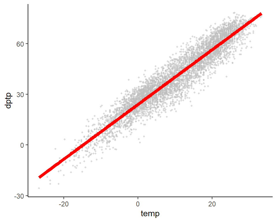

Plot some plots to check model assumptions for the model you fit using the autoplot function on your model object:

autoplot(mod_1)

7.8.5 Using regression models to explore data #2

Try fitting the regression from the last part of the in-course exercise as a GLM, using glm() (but still assuming the outcome variable is normally distributed). Are your coefficients different?
Does $PM_{10}$ vary by day of the week? (Hint: The dow variable is a factor that gives day of the week. You can do an ANOVA analysis by fitting a linear model using this variable as the independent variable. Some of the overall model summaries will compare this model to an intercept-only model.) What day of the week is $PM_{10}$ generally highest? (Check the model coefficients to figure this out.) Try to write out (on paper) the regression equation for the model you’re fitting.
Try using glm() to run a Poisson regression of respiratory deaths (resp) on temperature during summer days. Start by creating a subset with just summer days called summer. (Hint: Use the month function with the argument label = TRUE from lubridate to do this—just pull out the subset where the month June, July, or August.) Try to write out the regression equation for the model you’re fitting.
The coefficient for the temperature variable in this model is our best estimate (based on this model) of the log relative risk for a one degree Celcius increase in temperature. What is the relative risk associated with a one degree Celsius increase?

7.8.5.1 Example R code:

Try fitting the model from the last part of the in-course exercise using glm(). Call it mod_1a. Compare the coefficients for the two models. You can use the tidy function on an lm or glm object to pull out just the model coefficients and associated model results. Here, I’ve used a pipeline of code to create a tidy data frame that merges these “tidy” coefficient outputs (from the two models) into a single data frame):

mod_1a <- glm(dptp ~ temp, data = chic)

tidy(mod_1) %>% 
  select(term, estimate) %>% 
  inner_join(mod_1a %>% tidy() %>% select(term, estimate), by = "term") %>% 
  rename(estimate_lm_mod = estimate.x,
         estimate_glm_mod = estimate.y)

## # A tibble: 2 × 3
##   term        estimate_lm_mod estimate_glm_mod
##   <chr>                 <dbl>            <dbl>
## 1 (Intercept)           24.0             24.0 
## 2 temp                   1.62             1.62

The results from the two models are identical.

As a note, you could have also just run tidy on each model object, without merging them together into a single data frame:

tidy(mod_1)

## # A tibble: 2 × 5
##   term        estimate std.error statistic p.value
##   <chr>          <dbl>     <dbl>     <dbl>   <dbl>
## 1 (Intercept)    24.0    0.113        213.       0
## 2 temp            1.62   0.00763      212.       0

tidy(mod_1a)

## # A tibble: 2 × 5
##   term        estimate std.error statistic p.value
##   <chr>          <dbl>     <dbl>     <dbl>   <dbl>
## 1 (Intercept)    24.0    0.113        213.       0
## 2 temp            1.62   0.00763      212.       0

Fit a model of $PM_{10}$ regressed on day of week, where day of week is a factor.

mod_2 <- lm(pm10 ~ dow, data = chic)
tidy(mod_2)

## # A tibble: 7 × 5
##   term         estimate std.error statistic   p.value
##   <chr>           <dbl>     <dbl>     <dbl>     <dbl>
## 1 (Intercept)     27.5      0.730     37.7  7.47e-273
## 2 dowMonday        6.13     1.03       5.93 3.22e-  9
## 3 dowTuesday       6.80     1.03       6.62 4.05e- 11
## 4 dowWednesday     8.48     1.03       8.26 1.85e- 16
## 5 dowThursday      8.80     1.02       8.60 1.08e- 17
## 6 dowFriday        9.48     1.03       9.24 3.61e- 20
## 7 dowSaturday      3.66     1.03       3.56 3.68e-  4

Use glance to check some of the overall summaries of this model. The statistic column here is the F statistic from test comparing this model to an intercept-only model.

glance(mod_2)

## # A tibble: 1 × 12
##   r.squared adj.r.squared sigma statistic  p.value    df  logLik    AIC    BIC
##       <dbl>         <dbl> <dbl>     <dbl>    <dbl> <dbl>   <dbl>  <dbl>  <dbl>
## 1    0.0259        0.0247  19.1      21.5 4.61e-25     6 -21234. 42484. 42536.
## # ℹ 3 more variables: deviance <dbl>, df.residual <int>, nobs <int>

As a note, you may have heard in previous statistics classes that you can use the anova() command to compare this model to a model with only an intercept (i.e., one that only fits a global mean and uses that as the expected value for all of the observations). Note that, in this case, the F value from anova for this model comparison is the same as the statistic you got in the overall summary statistics you get with glance in the previous code.

anova(mod_2)

## Analysis of Variance Table
## 
## Response: pm10
##             Df  Sum Sq Mean Sq F value    Pr(>F)    
## dow          6   46924  7820.6    21.5 < 2.2e-16 ***
## Residuals 4856 1766407   363.8                      
## ---
## Signif. codes:  0 '***' 0.001 '**' 0.01 '*' 0.05 '.' 0.1 ' ' 1

The overall p-value from anova for with day-of-week coefficients versus the model that just has an intercept is < 2.2e-16. This is well below 0.05, which suggests that day-of-week is associated with PM10 concentration, as a model that includes day-of-week does a much better job of explaining variation in PM10 than a model without it does.

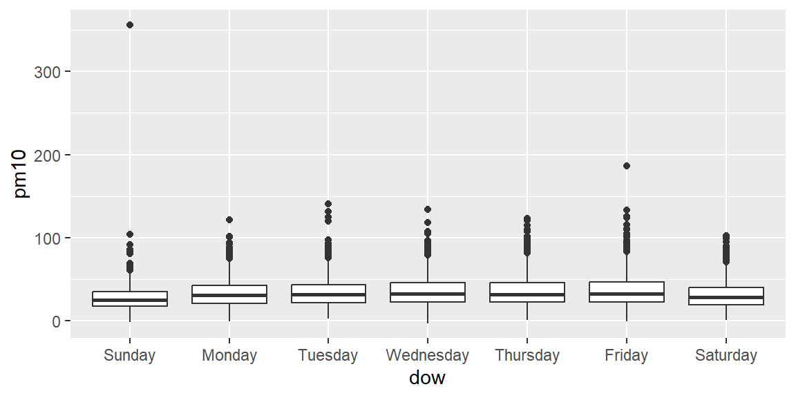
Use a boxplot to visually compare PM10 by day of week.

ggplot(chic, aes(x = dow, y = pm10)) + 
  geom_boxplot()

Now try the same plot, but try using the ylim = option to change the limits on the y-axis for the graph, so you can get a better idea of the pattern by day of week (some of the extreme values are very high, which makes it hard to compare by eye when the y-axis extends to include them all).

ggplot(chic, aes(x = dow, y = pm10)) + 
  geom_boxplot() + 
  ylim(c(0, 100))

## Warning: Removed 292 rows containing non-finite values (`stat_boxplot()`).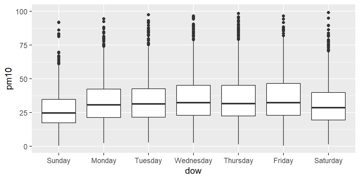

Create a subset called summer with just the summer days:

library(lubridate)
summer <- chic %>%
  mutate(month = month(date, label = TRUE)) %>% 
  filter(month %in% c("Jun", "Jul", "Aug"))
summer %>% 
  slice(1:3)

##         date time year month doy       dow death cvd resp     temp  dptp   rhum
## 1 1987-06-01  152 1987   Jun 152    Monday   112  60    5 23.61111 68.50 71.875
## 2 1987-06-02  153 1987   Jun 153   Tuesday   111  57    7 22.22222 64.75 95.250
## 3 1987-06-03  154 1987   Jun 154 Wednesday   120  59    9 20.55556 47.25 47.125
##       pm10       o3
## 1 22.95607 34.94623
## 2 31.31339 18.96620
## 3 34.95607 23.59270

Use glm() to fit a Poisson model of respiratory deaths regressed on temperature. Since you want to fit a Poisson model, use the option family = poisson(link = "log").

mod_3 <- glm(resp ~ temp, data = summer,
             family = poisson(link = "log"))
glance(mod_3)

## # A tibble: 1 × 8
##   null.deviance df.null logLik   AIC   BIC deviance df.residual  nobs
##           <dbl>   <int>  <dbl> <dbl> <dbl>    <dbl>       <int> <int>
## 1         1499.    1287 -3211. 6425. 6436.    1494.        1286  1288

tidy(mod_3)

## # A tibble: 2 × 5
##   term        estimate std.error statistic   p.value
##   <chr>          <dbl>     <dbl>     <dbl>     <dbl>
## 1 (Intercept)  1.91      0.0584      32.7  6.60e-235
## 2 temp         0.00614   0.00258      2.38 1.74e-  2

Use the fitted model coefficient to determine the relative risk for a one degree Celsius increase in temperature. First, remember that you can use the tidy() function to read out the model coefficients. The second of these is the value for the temperature coefficient. That means that you can use indexing ([2]) to get just that value. That’s the log relative risk; take the exponent to get the relative risk.

tidy(mod_3) %>% 
  filter(term == "temp") %>% 
  mutate(log_rr = exp(estimate))

## # A tibble: 1 × 6
##   term  estimate std.error statistic p.value log_rr
##   <chr>    <dbl>     <dbl>     <dbl>   <dbl>  <dbl>
## 1 temp   0.00614   0.00258      2.38  0.0174   1.01

As a note, you can use the conf.int parameter in tidy to also pull confidence intervals:

tidy(mod_3, conf.int = TRUE)

## # A tibble: 2 × 7
##   term        estimate std.error statistic   p.value conf.low conf.high
##   <chr>          <dbl>     <dbl>     <dbl>     <dbl>    <dbl>     <dbl>
## 1 (Intercept)  1.91      0.0584      32.7  6.60e-235  1.80       2.02  
## 2 temp         0.00614   0.00258      2.38 1.74e-  2  0.00108    0.0112

You could use this to get the confidence interval for relative risk (check out the mutate_at function if you haven’t seen it before):

tidy(mod_3, conf.int = TRUE) %>% 
  select(term, estimate, conf.low, conf.high) %>% 
  filter(term == "temp") %>% 
  mutate_at(vars(estimate:conf.high), funs(exp(.)))

## Warning: `funs()` was deprecated in dplyr 0.8.0.
## ℹ Please use a list of either functions or lambdas:
## 
## # Simple named list: list(mean = mean, median = median)
## 
## # Auto named with `tibble::lst()`: tibble::lst(mean, median)
## 
## # Using lambdas list(~ mean(., trim = .2), ~ median(., na.rm = TRUE))
## Call `lifecycle::last_lifecycle_warnings()` to see where this warning was
## generated.

## # A tibble: 1 × 4
##   term  estimate conf.low conf.high
##   <chr>    <dbl>    <dbl>     <dbl>
## 1 temp      1.01     1.00      1.01

7.8.6 Trying out nesting and mapping

We’ll be using data that’s in an R package called “nycflights13”. This data package can be installed from CRAN. Install the package and then load the package and its “flights” dataset. So that this data will be easier to work with, remove all columns except for those for the departure delay (dep_delay), the carrier (carrier), the hour the flight was supposed to leave (hour), and the airport the flight left from (origin). Also, limit the dataset to only flights that left from LaGuardia Airport (“LGA”).
We want to figure out if the probability of a flight leaving 15 minutes late or more increases over the day for flights leaving LaGuardia. Filter out all the rows where the departure delay is missing and then create a new column called late_dep that is true if the flight left 15 minutes or more late and false otherwise. What proportion of all flights leaving from LaGuardia leave 15 minutes late or later?
Next, determine what proportion of all flights are delayed base on the hour that the flight was scheduled to depart (hour). Create a plot showing how the probability of leaving 15 minutes or more late changes by hour.
Fit a generalized linear model for the association between the binary variable of whether the flight was 15 minutes or more late (late_dep) and the hour the flight was scheduled to leave (hour). Use a binomial model (add family = binomial(link = "logit") in the glm call). The estimate from the model for hour will be an estimate of the log odds ratio for a one-hour increase in scheduled departure time. Take the exponent of this estimate with exp to get an estimated odds ratio for a one-hour increase in scheduled departure time. Is this estimate larger than 1.0?
Next, we want to see if this association is similar across airlines. First, create a dataframe called nested_flights where the flights data is grouped by airline (carrier) and then nest the data, so that there is a “data” list-column where each item is a dataframe of flight delay data for a specific carrier.
Use the map function from purrr inside a mutate statement to apply the glm code you used earlier for the whole dataset, but in this case for the data for each airline character. Then use the map function inside a mutate statement again to “tidy” the data.
Clean the data up a bit. Remove the columns for data and glm_result and then unnest the dataframe list-column with the tidy version of the model results. Filter to get only the estimates for the “hour” term. Then calculate an odds ratio (or) by taking the exponent (check out the exp function) of the original estimate.
The package has a dataframe with the full name of each carrier (airlines). Join this data into the data you’ve been working with, so you have the full names of airlines.
Finally, create the following plot with each airline’s odds ratio for the change in the chance of a delay per one-hour increase in the scheduled hour of departure:

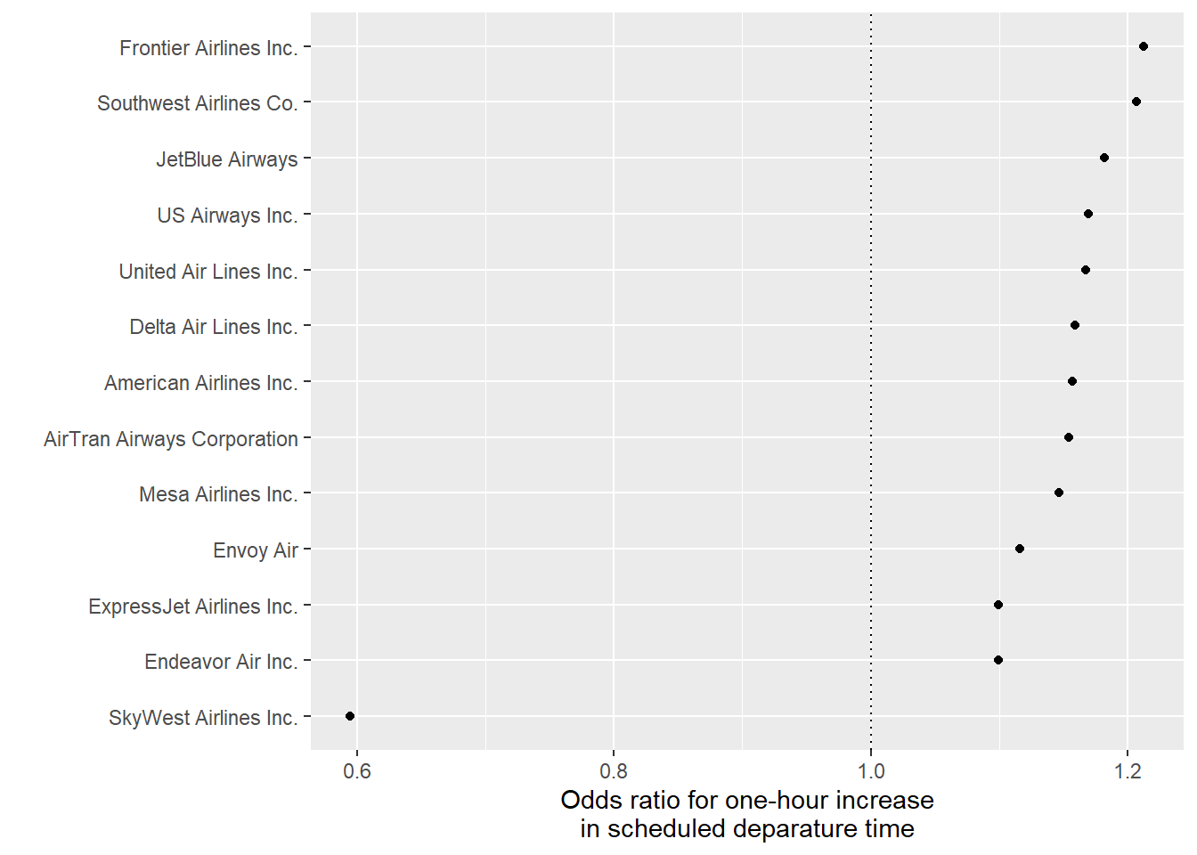
7.8.6.1 Example R code:

Install the “nycflights13” package from CRAN. Load the package and its “flights” dataset.

library(ggplot2)
library(nycflights13)
data(flights)

So that this data will be easier to work with, remove all columns except for those for the departure dealy (dep_delay), the carrier (carrier), the hour the flight was supposed to leave (hour), and the airport the flight left from (origin).

flights <- flights %>% 
  select(dep_delay, carrier, hour, origin) %>% 
  filter(origin == "LGA")

flights

## # A tibble: 104,662 × 4
##    dep_delay carrier  hour origin
##        <dbl> <chr>   <dbl> <chr> 
##  1         4 UA          5 LGA   
##  2        -6 DL          6 LGA   
##  3        -3 EV          6 LGA   
##  4        -2 AA          6 LGA   
##  5        -1 AA          6 LGA   
##  6         0 B6          6 LGA   
##  7         0 MQ          6 LGA   
##  8        -8 DL          6 LGA   
##  9        -3 MQ          6 LGA   
## 10        13 AA          6 LGA   
## # ℹ 104,652 more rows

Filter out all the rows where the departure delay is missing and then create a new column called late_dep that is true if the flight left 15 minutes or more late and false otherwise.

flights <- flights %>% 
  filter(!is.na(dep_delay)) %>% 
  mutate(late_dep = dep_delay > 15)

flights

## # A tibble: 101,509 × 5
##    dep_delay carrier  hour origin late_dep
##        <dbl> <chr>   <dbl> <chr>  <lgl>   
##  1         4 UA          5 LGA    FALSE   
##  2        -6 DL          6 LGA    FALSE   
##  3        -3 EV          6 LGA    FALSE   
##  4        -2 AA          6 LGA    FALSE   
##  5        -1 AA          6 LGA    FALSE   
##  6         0 B6          6 LGA    FALSE   
##  7         0 MQ          6 LGA    FALSE   
##  8        -8 DL          6 LGA    FALSE   
##  9        -3 MQ          6 LGA    FALSE   
## 10        13 AA          6 LGA    FALSE   
## # ℹ 101,499 more rows

What proportion of all flights leaving from LaGuardia leave 15 minutes late or later? To check this, remember that TRUE is saved as a “1” and FALSE is saved as a “0”. That means that we can take the mean of a logical vector to get the proportion of trials that are true.

flights %>% pull("late_dep") %>% mean()

## [1] 0.1889685

Determine what proportion of all flights are delayed base on the hour that the flight was scheduled to depart (hour). Create a plot showing how the probability of leaving 15 minutes or more late changes by hour.

flights_late <- flights %>% 
  group_by(hour) %>% 
  summarize(prob_late = mean(late_dep))

flights_late

## # A tibble: 18 × 2
##     hour prob_late
##    <dbl>     <dbl>
##  1     5    0.0588
##  2     6    0.0519
##  3     7    0.0570
##  4     8    0.0967
##  5     9    0.105 
##  6    10    0.128 
##  7    11    0.159 
##  8    12    0.163 
##  9    13    0.200 
## 10    14    0.207 
## 11    15    0.236 
## 12    16    0.273 
## 13    17    0.292 
## 14    18    0.298 
## 15    19    0.314 
## 16    20    0.331 
## 17    21    0.309 
## 18    22    0.391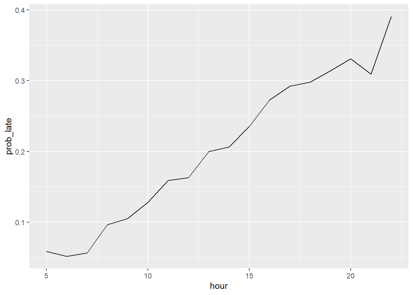

flights_late %>% 
  ggplot(aes(x = hour, y = prob_late)) + 
  geom_line()

Fit a generalized linear model for the association between the binary variable of whether the flight was 15 minutes or more late (late_dep) and the hour the flight was scheduled to leave (hour). Use a binomial model (add family = binomial(link = "logit") in the glm call). The estimate from the model for hour will be an estimate of the log odds ratio for a one-hour increase in scheduled departure time. Take the exponent of this estimate with exp to get an estimated odds ratio for a one-hour increase in scheduled departure time. Is this estimate larger than 1.0?

glm(late_dep ~ hour, data = flights, family = binomial(link = "logit"))

## 
## Call:  glm(formula = late_dep ~ hour, family = binomial(link = "logit"), 
##     data = flights)
## 
## Coefficients:
## (Intercept)         hour  
##     -3.3643       0.1399  
## 
## Degrees of Freedom: 101508 Total (i.e. Null);  101507 Residual
## Null Deviance:       98410 
## Residual Deviance: 92810     AIC: 92810

library(broom)
glm(late_dep ~ hour, data = flights, family = binomial(link = "logit")) %>% 
  tidy() %>%                 # Tidy the model results
  filter(term == "hour") %>% # Only look at the estimate for `hour`
  mutate(or = exp(estimate)) # Estimate is log odds ratio. Take exponent for odds ratio

## # A tibble: 1 × 6
##   term  estimate std.error statistic p.value    or
##   <chr>    <dbl>     <dbl>     <dbl>   <dbl> <dbl>
## 1 hour     0.140   0.00195      71.7       0  1.15

Next, we want to see if this association is similar across airlines. First, create a dataframe called nested_flights where the flights data is grouped by airline (carrier) and then nest the data, so that there is a “data” list-column where each item is a dataframe of flight delay data for a specific carrier:

nested_flights <- flights %>% 
  group_by(carrier) %>% 
  nest()

nested_flights

## # A tibble: 13 × 2
## # Groups:   carrier [13]
##    carrier data                 
##    <chr>   <list>               
##  1 UA      <tibble [7,837 × 4]> 
##  2 DL      <tibble [22,857 × 4]>
##  3 EV      <tibble [8,255 × 4]> 
##  4 AA      <tibble [15,063 × 4]>
##  5 B6      <tibble [5,925 × 4]> 
##  6 MQ      <tibble [16,189 × 4]>
##  7 WN      <tibble [6,000 × 4]> 
##  8 FL      <tibble [3,187 × 4]> 
##  9 US      <tibble [12,574 × 4]>
## 10 F9      <tibble [682 × 4]>   
## 11 9E      <tibble [2,372 × 4]> 
## 12 YV      <tibble [545 × 4]>   
## 13 OO      <tibble [23 × 4]>

To check the contents of the list-column, try:

nested_flights$data[[1]] %>% # Get the first element of the "data" column
  head()

## # A tibble: 6 × 4
##   dep_delay  hour origin late_dep
##       <dbl> <dbl> <chr>  <lgl>   
## 1         4     5 LGA    FALSE   
## 2        -4     6 LGA    FALSE   
## 3         1     6 LGA    FALSE   
## 4         9     7 LGA    FALSE   
## 5        -4     7 LGA    FALSE   
## 6         2     7 LGA    FALSE

Use the map function from purrr inside a mutate statement to apply the glm code you used earlier for the whole dataset, but in this case for the data for each airline character:

library(purrr)
library(tidyr)

prob_late <- nested_flights %>% 
  mutate(glm_result = purrr::map(data, ~ glm(late_dep ~ hour, 
                                      data = .x, family = binomial(link = "logit")))) 

# Check the results for the first element of the "glm_result" column: 
prob_late$glm_result[[1]]

## 
## Call:  glm(formula = late_dep ~ hour, family = binomial(link = "logit"), 
##     data = .x)
## 
## Coefficients:
## (Intercept)         hour  
##     -3.4305       0.1551  
## 
## Degrees of Freedom: 7836 Total (i.e. Null);  7835 Residual
## Null Deviance:       7601 
## Residual Deviance: 7064  AIC: 7068

Then use the map function inside a mutate statement again to “tidy” the data.

prob_late <- prob_late %>% 
  mutate(glm_tidy = purrr::map(glm_result, ~ tidy(.x)))

Remove the columns for data and glm_result:

prob_late <- prob_late %>% 
  select(-data, -glm_result)

Then `unnest the dataframe list-column with the tidy version of the model results:

prob_late <- prob_late %>% 
  unnest(glm_tidy)

Filter to get only the estimates for the “hour” term:

prob_late <- prob_late %>% 
  filter(term == "hour")

Then calculate an odds ratio (or) by taking the exponent (check the exp function) of the original estimate.

prob_late <- prob_late %>% 
  mutate(or = exp(estimate))
head(prob_late)

## # A tibble: 6 × 7
## # Groups:   carrier [6]
##   carrier term  estimate std.error statistic   p.value    or
##   <chr>   <chr>    <dbl>     <dbl>     <dbl>     <dbl> <dbl>
## 1 UA      hour    0.155    0.00705      22.0 2.88e-107  1.17
## 2 DL      hour    0.148    0.00454      32.6 1.80e-232  1.16
## 3 EV      hour    0.0952   0.00572      16.7 2.79e- 62  1.10
## 4 AA      hour    0.146    0.00580      25.2 1.05e-139  1.16
## 5 B6      hour    0.168    0.00702      23.9 7.13e-126  1.18
## 6 MQ      hour    0.110    0.00468      23.5 2.23e-122  1.12

The package has a dataframe with the full name of each carrier (airlines). Join this data into the data you’ve been working with, so you have the full names of airlines:

prob_late <- left_join(prob_late, airlines, by = "carrier")

Finally, create the following plot with each airline’s association between hour in the day and the chance of a delay:

library(forcats)
data(airlines)
prob_late %>% 
  ungroup() %>% 
  mutate(estimate = exp(estimate)) %>% 
  mutate(name = fct_reorder(name, estimate)) %>% 
  ggplot(aes(x = estimate, y = name)) + 
  geom_point() + 
  geom_vline(xintercept = 1, linetype = 3) + 
  labs(x = "Odds ratio for one-hour increase in scheduled deparature time", y = "")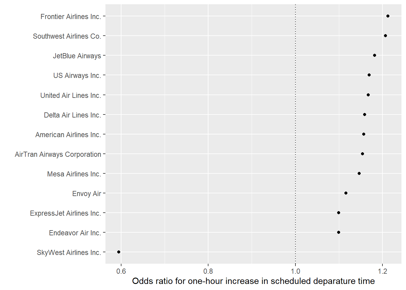

7.8.7 Writing functions

Say that you have a four-letter character string (e.g., “ling”) and that you want to move the last letter to the front of the string to create a new four-letter character string (e.g., “glin”). Write some R code to do this.
Next, write a function named move_letter that does the same thing—takes a four-letter character string (e.g., “ling”) and creates a new four-letter character string where the last letter in the original string has been moved to the front of the string (e.g., “glin”). It should input one parameter (word, the original four-letter character string or a vector of four-letter character strings).
Read the word list at https://raw.githubusercontent.com/dwyl/english-words/master/words.txt into an R dataframe called word_list. It will only have one column; name this column word.
Write code that can take a vector of character strings (e.g., c('ling', 'scat', 'soil')) and return a logical vector that says whether that character string is a word in the word_list dataframe you created in the last step (e.g., c('FALSE', 'TRUE', 'TRUE') for a vector where the first value isn’t a word but the second and third are). You may find the pull function useful in writing this code (to pull the word column out of the word_list dataframe).
Write a function called is_word that inputs (1) a vector of character strings and (2) a dataframe with a column called “word” that lists real words. The function should return a logical vector saying whether each character string is a real word. The function should have two arguments: words_to_check, which is a vector of character strings (e.g., c('ling', 'scat', 'soil')), and real_word_list, which is a dataframe with a column called words of real English words (e.g., the word_list dataframe you created from the word list on GitHub). Set the real_word_list argument to have the default value of words, the dataframe you created earlier in this exercise by reading in the dataframe of English words from GitHub.
Try using the function with a different word list. As an example, you could read in and use the word list of Google’s top 10,000 English words from https://raw.githubusercontent.com/first20hours/google-10000-english/master/google-10000-english-no-swears.txt.
Try using these functions to solve the word puzzle problem in the last homework.

7.8.7.1 Example R code

Say that you have a four-letter character string (e.g., “ling”) and that you want to move the last letter to the front of the string to create a new four-letter character string (e.g., “glin”). You can use functions from the stringr package to help with this.

library(stringr)

# Start with an example word. You can use the example word from 
# the problem statement ('ling').
word <- "ling"

# Break the word into two parts
first_three_letters <- str_sub(word, 1, 3)
last_letter <- str_sub(word, 4, 4)

first_three_letters

## [1] "lin"

last_letter

## [1] "g"

# Put the parts back together in the right order
new_word <- str_c(last_letter, first_three_letters) # You could also use `paste` or `paste0` here
new_word

## [1] "glin"

Write a function named move_letter that takes a four-letter character string (e.g., “ling”) and creates a new four-letter character string where the last letter in the original string has been moved to the front of the string (e.g., “glin”). It should input one parameter (word, the original four-letter character string or a vector of four-letter character strings).

To do this, take the code that you just wrote and put it inside a function named move_letter:

move_letter <- function(word){
  # Break the word into two parts
  first_three_letters <- str_sub(word, 1, 3)
  last_letter <- str_sub(word, 4, 4)
  
  # Put the parts back together in the right order
  str_c(last_letter, first_three_letters)
}

# Check the function
move_letter(word = "ling")

## [1] "glin"

# Try with some other four-letter strings
move_letter(word = "cats")

## [1] "scat"

move_letter(word = "oils")

## [1] "soil"

# Check using with a vector of four-letter character strings
move_letter(c("cats", "oils"))

## [1] "scat" "soil"

Notice that now word is being used as an argument in the function. It’s as if you assigned the string or vector of strings that you want to convert to the object name word, and then you run all the code. The output of the function is the last expression in the function code (str_c(last_letter, first_three_letters)). Also, note that you can add comments inside the function with #, just like you can with other R code.

Read the word list at https://raw.githubusercontent.com/dwyl/english-words/master/words.txt into an R dataframe called words. It will only have one column; name this column word_list.

library(readr)

word_list <- read_csv("https://raw.githubusercontent.com/dwyl/english-words/master/words.txt",
                  col_names = "word")

## Warning: One or more parsing issues, call `problems()` on your data frame for details,
## e.g.:
##   dat <- vroom(...)
##   problems(dat)

## Rows: 466550 Columns: 1
## ── Column specification ────────────────────────────────────────────────────────
## Delimiter: ","
## chr (1): word
## 
## ℹ Use `spec()` to retrieve the full column specification for this data.
## ℹ Specify the column types or set `show_col_types = FALSE` to quiet this message.

Write code that can take a vector of character strings (e.g., c('ling', 'scat', 'soil')) and return a logical vector that says whether that character string is a word in the word_list dataframe you created in the last step (e.g., c('TRUE', 'FALSE', 'TRUE') for a vector where the second value isn’t a word but the first and third are).

library(purrr)

words_to_check <- c("ling", "scat", "soil")
words_to_check %in% pull(word_list, "word")

## [1]  TRUE FALSE  TRUE

This code works because you can use pull to extract a column (as a vector) from a dataframe, and then you can use the %in% operator to see if each value in one vector (the words_to_check vector in this example) is one of the values in the second vector (the word column from the words dataframe in this example).

Write a function called is_word that inputs (1) a vector of character strings and (2) a dataframe with a column called “word” that lists real words. The function should return a logical vector saying whether each character string is a real word. The function should have two arguments: words_to_check, which is a vector of character strings and real_word_list which is a dataframe with a column called words of real English words. Set the real_word_list argument to have the default value of words, the dataframe you created earlier in this exercise by reading in the dataframe of English words from GitHub.

# Put the code you wrote inside a function
is_word <- function(words_to_check, real_word_list = word_list){
  words_to_check %in% pull(real_word_list, "word")
}

# Check the function
is_word(words_to_check = c("ling", "scat", "soil"))

## [1]  TRUE FALSE  TRUE

Note that, if you want to use the word_list dataframe for your real word list, you don’t have to specify that when you call the is_word function, since you set that as your default value.

If you wanted to use a different word list, you can specify a different value for the real_word_list argument when you run the function. For example, to use Google’s top 10,000 English word list from GitHub instead, use:

google_words <- read_csv("https://raw.githubusercontent.com/first20hours/google-10000-english/master/google-10000-english-no-swears.txt", 
                         col_names = "word")

## Rows: 9894 Columns: 1
## ── Column specification ────────────────────────────────────────────────────────
## Delimiter: ","
## chr (1): word
## 
## ℹ Use `spec()` to retrieve the full column specification for this data.
## ℹ Specify the column types or set `show_col_types = FALSE` to quiet this message.

is_word(words_to_check = c("ling", "scat", "soil"), real_word_list = google_words)

## [1] FALSE FALSE  TRUE

In this case, there was a rarer word (“ling”) that counted as a word when the original word list was used, but not when the Google top-10,000 words list was used.

Try using these functions to solve the word puzzle problem in the last homework.

word_list %>% 
  filter(str_detect(word, "^m.{7}$")) %>%                        # This is using regular expressions
  separate(word, into = c("first_word", "second_word"),          # Note that you can use `separate` with a number to use position
           sep = 4, remove = FALSE) %>%                          
  mutate(second_word = move_letter(second_word)) %>%             # Use the first function here
  filter(is_word(first_word) & is_word(second_word)) %>%         # Use the second function here
  unite("new_word", c("first_word", "second_word"), sep = " ")   # You can use `unite` to put the two new words in a phrase in one column.

## # A tibble: 103 × 2
##    word     new_word 
##    <chr>    <chr>    
##  1 mailings mail sing
##  2 maillots mail slot
##  3 majorate majo erat
##  4 majoring majo grin
##  5 malmiest malm ties
##  6 maltiest malt ties
##  7 mandalas mand sala
##  8 mandated mand date
##  9 mandates mand sate
## 10 mangiest mang ties
## # ℹ 93 more rows

You can get the choices down to even fewer options if you match the new words against the Google top-10,000 words list, by using the real_word_list option in the is_word function you wrote. (However, “maillots” is not a common enough word that you can also start from that shorter word list!)

word_list %>% 
  filter(str_detect(word, "^m.{7}$")) %>%                        
  separate(word, into = c("first_word", "second_word"),          
           sep = 4, remove = FALSE) %>%                          
  mutate(second_word = move_letter(second_word)) %>%             
  filter(is_word(first_word, real_word_list = google_words) & 
           is_word(second_word, real_word_list = google_words)) %>%         
  unite("new_word", c("first_word", "second_word"), sep = " ")

## # A tibble: 43 × 2
##    word     new_word 
##    <chr>    <chr>    
##  1 mailings mail sing
##  2 maillots mail slot
##  3 maintops main stop
##  4 markings mark sing
##  5 maskings mask sing
##  6 massager mass rage
##  7 massages mass sage
##  8 massiest mass ties
##  9 mattings matt sing
## 10 mealiest meal ties
## # ℹ 33 more rows