Chapter 5 Reproducible research #1

The video lectures for this chapter are embedded at relevant places in the text, with links to download a pdf of the associated slides for each video. You can also access a full playlist for the videos for this chapter.

5.1 What is reproducible research?

Download a pdf of the lecture slides for this video.

A data analysis is reproducible if all the information (data, files, etc.) required is available for someone else to re-do your entire analysis. This includes:

Data available
All code for cleaning raw data
All code and software (specific versions, packages) for analysis

Some advantages of making your research reproducible are:

You can (easily) figure out what you did six months from now.
You can (easily) make adjustments to code or data, even early in the process, and re-run all analysis.
When you’re ready to publish, you can (easily) do a last double-check of your full analysis, from cleaning the raw data through generating figures and tables for the paper.
You can pass along or share a project with others.
You can give useful code examples to people who want to extend your research.

Here is a famous research example of the dangers of writing code that is hard to double-check or confirm:

Some of the steps required to making research reproducible are:

All your raw data should be saved in the project directory. You should have clear documentation on the source of all this data.
Scripts should be included with all the code used to clean this data into the data set(s) used for final analyses and to create any figures and tables.
You should include details on the versions of any software used in analysis (for R, this includes the version of R as well as versions of all packages used).
If possible, there should be no “by hand” steps used in the analysis; instead, all steps should be done using code saved in scripts. For example, you should use a script to clean data, rather than cleaning it by hand in Excel. If any “non-scriptable” steps are unavoidable, you should very clearly document those steps.

There are several software tools that can help you improve the reproducibility of your research:

knitr: Create files that include both your code and text. These can be rendered to create final reports and papers. They keep code within the final file for the report.
knitr complements: Create fancier tables and figures within RMarkdown documents. Packages include tikzDevice, animate, xtables, and pander.
packrat: Save versions of each package used for the analysis, then load those package versions when code is run again in the future.

In this section, I will focus on using knitr and RMarkdown files.

5.2 Markdown

Download a pdf of the lecture slides for this video.

R Markdown files are mostly written using Markdown. To write R Markdown files, you need to understand what markup languages like Markdown are and how they work.

In Word and other word processing programs you have used, you can add formatting using buttons and keyboard shortcuts (e.g., “Ctrl-B” for bold). The file saves the words you type. It also saves the formatting, but you see the final output, rather than the formatting markup, when you edit the file (WYSIWYG – what you see is what you get).

In markup languages, on the other hand, you markup the document directly to show what formatting the final version should have (e.g., you type **bold** in the file to end up with a document with bold).

Examples of markup languages include:

HTML (HyperText Markup Language)
LaTex
Markdown (a “lightweight” markup language)

For example, Figure 5.1 some marked-up HTML code from CSU’s website, while Figure 5.2 shows how that file looks when it’s rendered by a web browser.

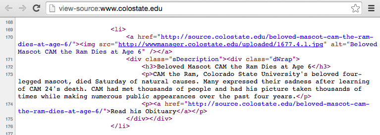
Figure 5.1: Example of the source of an HTML file.

Figure 5.2: Example of a rendered HTML file.

To write a file in Markdown, you’ll need to learn the conventions for creating formatting. This table shows what you would need to write in a flat file for some common formatting choices:

Code	Rendering	Explanation
`text`	text	boldface
`text`	text	italicized
`[text](www.google.com)`	text	hyperlink
`# text`		first-level header
`## text`		second-level header

Some other simple things you can do in Markdown include:

Lists (ordered or bulleted)
Equations
Tables
Figures from file
Block quotes
Superscripts

For more Markdown conventions, see RStudio’s R Markdown Reference Guide (link also available through “Help” in RStudio).

5.3 Literate programming in R

Download a pdf of the lecture slides for this video.

Literate programming, an idea developed by Donald Knuth, mixes code that can be executed with regular text. The files you create can then be rendered, to run any embedded code. The final output will have results from your code and the regular text.

The knitr package can be used for literate programming in R. In essence, knitr allows you to write an R Markdown file that can be rendered into a pdf, Word, or HTML document.

Here are the basics of opening and rendering an R Markdown file in RStudio:

To open a new R Markdown file, go to “File” -> “New File” -> “RMarkdown…” -> for now, chose a “Document” in “HTML” format.
This will open a new R Markdown file in RStudio. The file extension for R Markdown files is “.Rmd”.
The new file comes with some example code and text. You can run the file as-is to try out the example. You will ultimately delete this example code and text and replace it with your own.
Once you “knit” the R Markdown file, R will render an HTML file with the output. This is automatically saved in the same directory where you saved your .Rmd file.
Write everything besides R code using Markdown syntax.

To include R code in an RMarkdown document, you need to separate off the code chunk using the following syntax:

```{r}
my_vec <- 1:10
```

This syntax tells R how to find the start and end of pieces of R code when the file is rendered. R will walk through, find each piece of R code, run it and create output (printed output or figures, for example), and then pass the file along to another program to complete rendering (e.g., Tex for pdf files).

You can specify a name for each chunk, if you’d like, by including it after “r” when you begin your chunk. For example, to give the name load_nepali to a code chunk that loads the nepali dataset, specify that name in the start of the code chunk:

```{r load_nepali}
library(faraway)
data(nepali)
```

Here are a couple of tips for naming code chunks:

Chunk names must be unique across a document.
Any chunks you don’t name are given numbers by knitr.

You do not have to name each chunk. However, there are some advantages:

It will be easier to find any errors.
You can use the chunk labels in referencing for figure labels.
You can reference chunks later by name.

You can add options when you start a chunk. Many of these options can be set as TRUE / FALSE and include:

Option	Action
`echo`	Print out the R code?
`eval`	Run the R code?
`messages`	Print out messages?
`warnings`	Print out warnings?
`include`	If FALSE, run code, but don’t print code or results

Other chunk options take values other than TRUE / FALSE. Some you might want to include are:

Option	Action
`results`	How to print results (e.g., `hide` runs the code, but doesn’t print the results)
`fig.width`	Width to print your figure, in inches (e.g., `fig.width = 4`)
`fig.height`	Height to print your figure

Add these options in the opening brackets and separate multiple ones with commas:

```{r  messages = FALSE, echo = FALSE}
nepali[1, 1:3]
```

I will cover other chunk options later, once you’ve gotten the chance to try writting R Markdown files.

You can set “global” options at the beginning of the document. This will create new defaults for all of the chunks in the document. For example, if you want echo, warning, and message to be FALSE by default in all code chunks, you can run:

```{r  global_options}
knitr::opts_chunk$set(echo = FALSE, message = FALSE,
  warning = FALSE)
```

If you set both global and local chunk options that you set specifically for a chunk will take precedence over global options. For example, running a document with:

```{r  global_options}
knitr::opts_chunk$set(echo = FALSE, message = FALSE,
  warning = FALSE)
```


```{r  check_nepali, echo = TRUE}
head(nepali, 1)
```

would print the code for the check_nepali chunk, because the option specified for that specific chunk (echo = TRUE) would override the global option (echo = FALSE).

You can also include R output directly in your text (“inline”) using backticks:

“There are `r nrow(nepali)` observations in the nepali data set. The average age is `r mean(nepali$age, na.rm = TRUE)` months.”

Once the file is rendered, this gives:

“There are 1000 observations in the nepali data set. The average age is 37.662 months.”

Download a pdf of the lecture slides for this video.

Here are two tips that will help you diagnose some problems rendering R Markdown files:

Be sure to save your R Markdown file before you run it.
All the code in the file will run “from scratch”– as if you just opened a new R session.
The code will run using, as a working directory, the directory where you saved the R Markdown file.

You’ll want to try out pieces of your code as you write an R Markdown document. There are a few ways you can do that:

You can run code in chunks just like you can run code from a script (Ctrl-Return or the “Run” button).
You can run all the code in a chunk (or all the code in all chunks) using the different options under the “Run” button in RStudio.
All the “Run” options have keyboard shortcuts, so you can use those.

You can render R Markdown documents to other formats:

Word
Pdf (requires that you’ve installed “Tex” on your computer.)
Slides (ioslides)

Click the button to the right of “Knit” to see different options for rendering on your computer.

You can freely post your RMarkdown documents at RPubs. If you want to post to RPubs, you need to create an account. Once you do, you can click the “Publish” button on the window that pops up with your rendered file. RPubs can also be a great place to look for interesting example code, although it sometimes can be pretty overwhelmed with MOOC homework.

If you’d like to find out more, here are two good how-to books on reproducible research in R (the CSU library has both in hard copy):

Reproducible Research with R and RStudio, Christopher Gandrud
Dynamic Documents with R and knitr, Yihui Xie

5.4 Style guidelines

Download a pdf of the lecture slides for this video.

R style guidelines provide rules for how to format code in an R script. Some people develop their own style as they learn to code. However, it is easy to get in the habit of following style guidelines, and they offer some important advantages:

Clean code is easier to read and interpret later.
It’s easier to catch and fix mistakes when code is clear.
Others can more easily follow and adapt your code if it’s clean.
Some style guidelines will help prevent possible problems (e.g., avoiding . in function names).

For this course, we will use R style guidelines from two sources:

These two sets of style guidelines are very similar.

Hear are a few guidelines we’ve already covered in class:

Use <-, not =, for assignment.
Guidelines for naming objects:
- All lowercase letters or numbers
- Use underscore (_) to separate words, not camelCase or a dot (.) (this differs for Google and Wickham style guides)
- Have some consistent names to use for “throw-away” objects (e.g., df, ex, a, b)
Make names meaningful
- Descriptive names for R scripts (“random_group_assignment.R”)
- Nouns for objects (todays_groups for an object with group assignments)
- Verbs for functions (make_groups for the function to assign groups)

5.4.1 Line length

Google: Keep lines to 80 characters or less

To set your script pane to be limited to 80 characters, go to “RStudio” -> “Preferences” -> “Code” -> “Display”, and set “Margin Column” to 80.

# Do
my_df <- data.frame(n = 1:3,
                    letter = c("a", "b", "c"),
                    cap_letter = c("A", "B", "C"))

# Don't
my_df <- data.frame(n = 1:3, letter = c("a", "b", "c"), cap_letter = c("A", "B", "C"))

This guideline helps ensure that your code is formatted in a way that you can see all of the code without scrolling horizontally (left and right).

5.4.2 Spacing

Binary operators (e.g., <-, +, -) should have a space on either side
A comma should have a space after it, but not before.
Colons should not have a space on either side.
Put spaces before and after = when assigning parameter arguments

# Do
shots_per_min <- worldcup$Shots / worldcup$Time
#Don't 
shots_per_min<-worldcup$Shots/worldcup$Time

#Do
ave_time <- mean(worldcup[1:10 , "Time"])
#Don't
ave_time<-mean(worldcup[1 : 10 ,"Time"])

5.4.3 Semicolons

Although you can use a semicolon to put two lines of code on the same line, you should avoid it.

# Do
a <- 1:10
b <- 3

# Don't
a <- 1:10; b <- 3

5.4.4 Commenting

For a comment on its own line, use #. Follow with a space, then the comment.
You can put a short comment at the end of a line of R code. In this case, put two spaces after the end of the code, one #, and one more space before the comment.
If it helps make it easier to read your code, separate sections using a comment character followed by many hyphens (e.g., #------------). Anything after the comment character is “muted”.

# Read in health data ---------------------------

# Clean exposure data ---------------------------

5.4.5 Indentation

Google:

Within function calls, line up new lines with first letter after opening parenthesis for parameters to function calls:

Example:

# Relabel sex variable
nepali$sex <- factor(nepali$sex, 
                     levels = c(1, 2),
                     labels = c("Male", "Female"))

5.4.6 Code grouping

Group related pieces of code together.
Separate blocks of code by empty spaces.

# Load data
library(faraway)
data(nepali)

# Relabel sex variable
nepali$sex <- factor(nepali$sex, 
                     levels = c(1, 2),
                     labels = c("Male", "Female"))

Note that this grouping often happens naturally when using tidyverse functions, since they encourage piping (%>% and +).

5.4.7 Broader guidelines

Omit needless code.
Don’t repeat yourself.

We’ll learn more about satisfying these guidelines when we talk about writing your own functions in the next part of the class.

5.5 More with knitr

Download a pdf of the lecture slides for this video.

5.5.1 Equations in `knitr`

You can write equations in RMarkdown documents by setting them apart with dollar signs ($). For an equation on a line by itself (display equation), you two $s before and after the equation, on separate lines, then use LaTex syntax for writing the equations.

To help with this, you may want to use this LaTex math cheat sheet.. You may also find an online LaTex equation editor like Codecogs.com helpful.

Note: Equations denoted this way will always compile for pdf documents, but won’t always come through on Markdown files (for example, GitHub won’t compile math equations).

For example, writing this in your R Markdown file:

$$
E(Y_{t}) \sim \beta_{0} + \beta_{1}X_{1}
$$

will result in this rendered equation:

\[ E(Y_{t}) \sim \beta_{0} + \beta_{1}X_{1} \]

To put math within a sentence (inline equation), just use one $ on either side of the math. For example, writing this in a R Markdown file:

"We are trying to model $E(Y_{t})$."

The rendered document will show up as:

“We are trying to model $E(Y_{t})$.”

5.5.2 Figures from file

You can include not only figures that you create with R, but also figures that you have saved on your computer.

The best way to do that is with the include_graphics function in knitr:

library(knitr)
include_graphics("figures/CSU_ram.png")

This example would include a figure with the filename “MyFigure.png” that is saved in the “figures” sub-directory of the parent directory of the directory where your .Rmd is saved. Don’t forget that you will need to give an absolute pathway or the relative pathway from the directory where the .Rmd file is saved.

5.5.3 Saving graphics files

You can save figures that you create in R. Typically, you won’t need to save figures for an R Markdown file, since you can include figure code directly. However, you will sometimes want to save a figure from a script. You have two options:

Use the “Export” choice in RStudio
Write code to export the figure in your R script

To make your research more reproducible, use the second choice.

To use code export a figure you created in R, take three steps:

Open a graphics device (e.g., pdf("MyFile.pdf")).
Write the code to print your plot.
Close the graphics device using dev.off().

For example, the following code would save a scatterplot of time versus passes as a pdf named “MyFigure” in the “figures” subdirectory of the current working directory:

pdf("figures/MyFigure.pdf", width = 8, height = 6)
ggplot(worldcup, aes(x = Time, y = Passes)) + 
        geom_point(aes(color = Position)) + 
        theme_bw()
dev.off()

If you create multiple plots before you close the device, they’ll all save to different pages of the same pdf file.

You can open a number of different graphics devices. Here are some of the functions you can use to open graphics devices:

pdf
png
bmp
jpeg
tiff
svg

You will use a device-specific function to open a graphics device (e.g., pdf). However, you will always close these devices with dev.off.

Most of the functions to open graphics devices include parameters like height and width. These can be used to specify the size of the output figure. The units for these depend on the device (e.g., inches for pdf, pixels by default for png). Use the helpfile for the function to determine these details.

5.5.4 Tables in R Markdown

If you want to create a nice, formatted table from an R dataframe, you can do that using kable from the knitr package.

my_df <- data.frame(letters = c("a", "b", "c"),
                    numbers = 1:3)
kable(my_df)

letters	numbers
a	1
b	2
c	3

There are a few options for the kable function:

arg	expl
`colnames`	Column names (default: column name in the dataframe)
`align`	A vector giving the alignment for each column (‘l’, ‘c’, ‘r’)
`caption`	Table caption
`digits`	Number of digits to round to. If you want to round columns different amounts, use a vector with one element for each column.

my.df <- data.frame(letters = c("a", "b", "c"),
                numbers = rnorm(3))
kable(my.df, digits = 2, align = c("r", "c"),
      caption = "My new table", 
      col.names = c("First 3 letters", 
                    "First 3 numbers"))

Table 5.1: My new table
First 3 letters	First 3 numbers
a	-1.13
b	0.21
c	-0.21

From Yihui:

“Want more features? No, that is all I have. You should turn to other packages for help. I’m not going to reinvent their wheels.”

If you want to do fancier tables, you may want to explore the xtable and pander packages. As a note, these might both be more effective when compiling to pdf, rather than html.

5.6 In-course exercise Chapter 5

For all of today’s tasks, you’ll use the code from last week’s in-course exercise to do the exercises. This week we are not focusing on writing new code, but rather on how to take R code and put it in an R Markdown file, so we can create reports from files that include the original code.

5.6.1 Creating a Markdown document

First, you’ll create a Markdown document, without any R code in it yet.

In RStudio, go to “File” -> “New File” -> “R Markdown”. From the window that brings up, choose “Document” on the left-hand column and “HTML” as the output format. A new file will open in the script pane of your RStudio session. Save this file (you may pick the name and directory). The file extension should be “.Rmd”.

First, before you try to write your own Markdown, try rendering the example that the script includes by default. (This code is always included, as a template, when you first open a new RMarkdown file using the RStudio “New file” interface we used in this example.) Try rendering this default R Markdown example by clicking the “Knit” button at the top of the script file.

For some of you, you may not yet have everything you need on your computer to be able to get this to work. If so, let me know. RStudio usually includes all the necessary tools when you install it, but there may be some exceptions.

If you could get the document to knit, do the following tasks:

Look through the HTML document that was created. Compare it to the R Markdown script that created it, and see if you can understand, at least broadly, what’s going on.
Look in the directory where you saved the R Markdown file. You should now also see a new, .html file in that folder. Try opening it with a web browser like Safari.
Go back to the R Markdown file. Delete everything after the initial header information (everything after the 6th line). In the header information, make sure the title, author, and date are things you’re happy with. If not, change them.
Using Markdown syntax, write up a description of the data (worldcup) we used last week to create the fancier figure. Try to include the following elements:
- Bold and italic text
- Hyperlinks
- A list, either ordered or bulleted
- Headers

5.6.2 Adding in R code

Now incorporate the R code from previous weeks’ exercises into your document. Once you get the document to render with some basic pieces of code in it, try the following:

Try some different chunk options. For example, try setting echo = FALSE in some of your code chunks. Similarly, try using the options results = "hide" and include = FALSE.
You should have at least one code chunk that generates figures. Try experimenting with the fig.width and fig.height options for the chunk to change the size of the figure.
Try using the global commands. See if you can switch the echo default value for this document from TRUE (the usual default) to FALSE.

5.6.3 Working with R Markdown documents

Finally, try the following tasks to get some experience working with R Markdown files in RStudio:

Go to one of your code chunks. Locate the small gray arrow just to the left of the line where you initiate the code chunk. Click on it and see what happens. Then click on it again.
Put your cursor inside one of your code chunks. Try using the “Run” button (or Ctrl-Return) to run code in that chunk at your R console. Did it work?
Pick a code chunk in your document. Put your cursor somewhere in the code in that chunk. Click on the “Run” button and choose “Run All Chunks Above”. What did that do? If it did not work, what do you think might be going on? (Hint: Check getwd() and think about which directory you’ve used to save your R Markdown file.)
Pick another chunk of code. Put the cursor somewhere in the code for that chunk. Click on the “Run” button and choose “Run Current Chunk”. Then try “Run Next Chunk”. Try to figure out all the options the “Run” button gives you and when each might be useful.
Click on the small gray arrow to the right of the “Knit HTML” button. If the option is offered, select “Knit Word” and try it. What does this do?

5.6.4 R style guidelines

Go through all the R code in your R Markdown file. Are there are places where your code is not following style conventions for R? Clean up your code to correct any of these issues.

Chapter 5 Reproducible research #1

5.1 What is reproducible research?

5.2 Markdown

5.3 Literate programming in R

5.4 Style guidelines

5.4.1 Line length

5.4.2 Spacing

5.4.3 Semicolons

5.4.4 Commenting

5.4.5 Indentation

5.4.6 Code grouping

5.4.7 Broader guidelines

5.5 More with knitr

5.5.1 Equations in knitr

5.5.2 Figures from file

5.5.3 Saving graphics files

5.5.4 Tables in R Markdown

5.6 In-course exercise Chapter 5

5.6.1 Creating a Markdown document

5.6.2 Adding in R code

5.6.3 Working with R Markdown documents

5.6.4 R style guidelines

5.5.1 Equations in `knitr`