Chapter 6 Entering and cleaning data #2

The video lectures for this chapter are embedded at relevant places in the text, with links to download a pdf of the associated slides for each video. You can also access a full playlist for the videos for this chapter.

6.1 Tidy data

Download a pdf of the lecture slides for this video.

All of the material in this section comes directly from Hadley Wickham’s paper on tidy data. You will need to read this paper to prepare for the quiz on this section.

Getting your data into a “tidy” format makes it easier to model and plot. By taking the time to tidy your data at the start of an analysis, you will save yourself time, and make it easier to plan out later steps.

Characteristics of tidy data are:

1. Each variable forms a column.
2. Each observation forms a row.
3. Each type of observational unit forms a table.

Here are five common problems that Hadley Wickham has identified that keep data from being tidy:

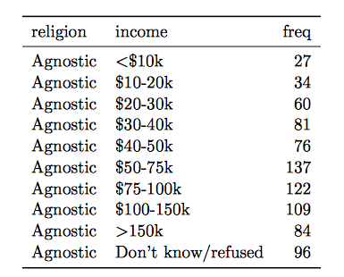
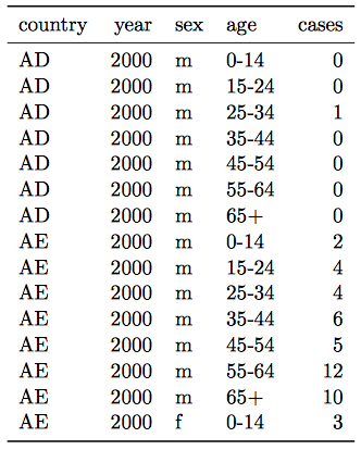
1. Column headers are values, not variable names.
2. Multiple variables are stored in one column.
3. Variables are stored in both rows and columns.
4. Multiple types of observational units are stored in the same table.
5. A single observational unit is stored in multiple tables.

Here are examples (again, from Hadley Wickham’s paper on tidy data, which is required reading for this week of the course) of each of these problems.

1. Column headers are values, not variable names.

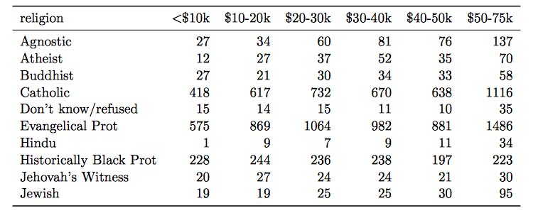
Solution:

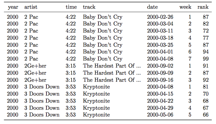
2. Multiple variables are stored in one column.

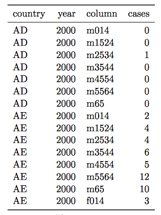
Solution:

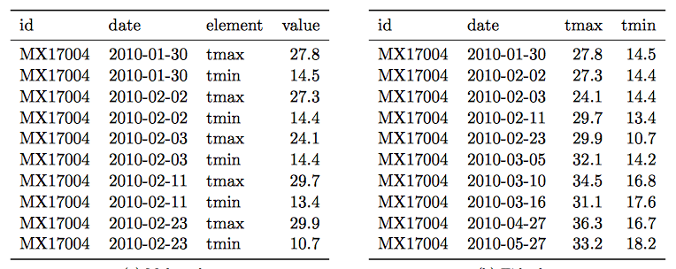
3. Variables are stored in both rows and columns.

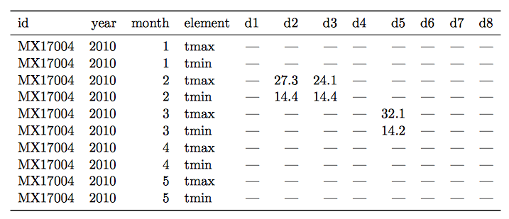
Solution:

4. Multiple types of observational units are stored in the same table.

Solution:

5. A single observational unit is stored in multiple tables.

Example: exposure and outcome data stored in different files:

• File 1: Daily mortality counts
• File 2: Daily air pollution measurements

6.2 Joining datasets

Download a pdf of the lecture slides for this video.

So far, you have only worked with a single data source at a time. When you work on your own projects, however, you typically will need to merge together two or more datasets to create the a data frame to answer your research question. For example, for air pollution epidemiology, you will often have to join several datasets:

• Health outcome data (e.g., number of deaths per day)
• Air pollution concentrations
• Weather measurements (since weather can be a confounder)
• Demographic data

The dplyr package has a family of different functions to join two dataframes together, the *_join family of functions. All combine two dataframes, which I’ll call x and y here.

The functions include:

• inner_join(x, y): Keep only rows where there are observations in both x and y.
• left_join(x, y): Keep all rows from x, whether they have a match in y or not.
• right_join(x, y): Keep all rows from y, whether they have a match in x or not.
• full_join(x, y): Keep all rows from both x and y, whether they have a match in the other dataset or not.

In the examples, I’ll use two datasets, x and y. Both datasets include the column course. The other column in x is grade, while the other column in y is day. Observations exist for courses x and y in both datasets, but for w and z in only one dataset.

x <- data.frame(course = c("x", "y", "z"),
                grade = c(90, 82, 78))
y <- data.frame(course = c("w", "x", "y"),
                day = c("Tues", "Mon / Fri", "Tue"))

Here is what these two example datasets look like:

x

##   course grade
## 1      x    90
## 2      y    82
## 3      z    78

y

##   course       day
## 1      w      Tues
## 2      x Mon / Fri
## 3      y       Tue

With inner_join, you’ll only get the observations that show up in both datasets. That means you’ll lose data on z (only in the first dataset) and w (only in the second dataset).

inner_join(x, y)

## Joining with `by = join_by(course)`

##   course grade       day
## 1      x    90 Mon / Fri
## 2      y    82       Tue

With left_join, you’ll keep everything in x (the “left” dataset), but not keep things in y that don’t match something in x. That means that, here, you’ll lose w:

left_join(x, y)

## Joining with `by = join_by(course)`

##   course grade       day
## 1      x    90 Mon / Fri
## 2      y    82       Tue
## 3      z    78      <NA>

right_join is the opposite:

right_join(x, y)

## Joining with `by = join_by(course)`

##   course grade       day
## 1      x    90 Mon / Fri
## 2      y    82       Tue
## 3      w    NA      Tues

full_join keeps everything from both datasets:

full_join(x, y)

## Joining with `by = join_by(course)`

##   course grade       day
## 1      x    90 Mon / Fri
## 2      y    82       Tue
## 3      z    78      <NA>
## 4      w    NA      Tues

6.3 Longer data

Download a pdf of the lecture slides for this video.

There are two functions from the tidyr package (another member of the tidyverse) that you can use to change between wider and longr data: pivot_longer and pivot_wider. Here is a description of these two functions:

• pivot_longer: Takes several columns and pivots them down into two columns. One of the new columns contains the former column names and the other contains the former cell values.
• pivot_wider: Takes two columns and pivots them up into multiple columns. Column names for the new columns will come from one column and the cell values from the other.

The following examples are show the effects of making a dataset longer or wider.

Here is some simulated wide data:

wide_stocks[1:3, ]

## # A tibble: 3 × 4
##   time             X      Y      Z
##   <date>       <dbl>  <dbl>  <dbl>
## 1 2009-01-01 -0.220   0.604 -6.90 
## 2 2009-01-02 -0.0971  0.673 -7.56 
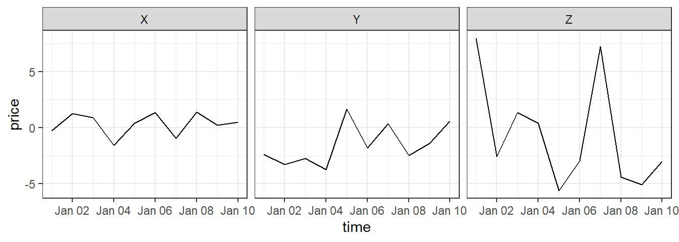
## 3 2009-01-03 -0.120  -2.92  -0.714

In the wide_stocks dataset, there are separate columns for three different stocks (X, Y, and Z). Each cell gives the value for a certain stock on a certain day. This data isn’t “tidy”, because the identify of the stock (X, Y, or Z) is a variable, and you’ll probably want to include it as a variable in modeling.

wide_stocks[1:3, ]

## # A tibble: 3 × 4
##   time             X      Y      Z
##   <date>       <dbl>  <dbl>  <dbl>
## 1 2009-01-01 -0.220   0.604 -6.90 
## 2 2009-01-02 -0.0971  0.673 -7.56 
## 3 2009-01-03 -0.120  -2.92  -0.714

If you want to convert the dataframe to have all stock values in a single column, you can use pivot_longer to convert wide data to long data:

long_stocks <- pivot_longer(data = wide_stocks,
                            cols = -time,
                            names_to = "stock",
                            values_to = "price")
long_stocks[1:5, ]

## # A tibble: 5 × 3
##   time       stock   price
##   <date>     <chr>   <dbl>
## 1 2009-01-01 X     -0.220 
## 2 2009-01-01 Y      0.604 
## 3 2009-01-01 Z     -6.90  
## 4 2009-01-02 X     -0.0971
## 5 2009-01-02 Y      0.673

In this “longer” dataframe, there is now one column that gives the identify of the stock (stock) and another column that gives the price of that stock that day (price):

long_stocks[1:5, ]

## # A tibble: 5 × 3
##   time       stock   price
##   <date>     <chr>   <dbl>
## 1 2009-01-01 X     -0.220 
## 2 2009-01-01 Y      0.604 
## 3 2009-01-01 Z     -6.90  
## 4 2009-01-02 X     -0.0971
## 5 2009-01-02 Y      0.673

The format for a pivots_longer call is:

## Generic code
new_df <- pivot_longer(old_df,
                       cols = [name(s) of the columns you want to make longer],
                       names_to = [name of new column to store the old column names],
                       values_to = [name of new column to store the old values])

Three important notes:

• Everything is pivoted into one of two columns – one column with the old column names, and one column with the old cell values
• With the names_to and values_to arguments, you are just providing column names for the two columns that everything’s pivoted into.
• If there is a column you don’t want to include in the pivot (date in the example), use - to exclude it in the cols argument.

Notice how easy it is, now that the data is longer, to use stock for aesthetics of faceting in a ggplot2 call:

ggplot(long_stocks, aes(x = time, y = price)) + 
  geom_line() + 
  facet_grid(. ~ stock) +
  theme_bw()

If you have data in a “longer” format and would like to make it “wider”, you can use pivot_wider to do that:

stocks <- pivot_wider(long_stocks,
                      names_from = "stock",
                      values_from = price)
stocks[1:5, ]

## # A tibble: 5 × 4
##   time             X      Y      Z
##   <date>       <dbl>  <dbl>  <dbl>
## 1 2009-01-01 -0.220   0.604 -6.90 
## 2 2009-01-02 -0.0971  0.673 -7.56 
## 3 2009-01-03 -0.120  -2.92  -0.714
## 4 2009-01-04  0.667   0.553 -5.52 
## 5 2009-01-05  0.431   0.692  6.57

Notice that this reverses the action of pivot_longer.

The “wider” your data the less likely it is to be tidy, so won’t use pivot_wider frequently when you are preparing data for analysis. However, pivot_wider can be very helpful in creating tables for final reports and presentations.

For example, if you wanted to create a table with means and standard deviations for each of the three stocks, you could use pivot_wider to rearrange the final summary to create an attractive table.

stock_summary <- long_stocks %>% 
  group_by(stock) %>%
  summarize(N = n(), mean = mean(price), sd = sd(price))
stock_summary

## # A tibble: 3 × 4
##   stock     N   mean    sd
##   <chr> <int>  <dbl> <dbl>
## 1 X        10  0.288 0.889
## 2 Y        10  0.191 1.78 
## 3 Z        10 -0.264 5.26

stock_summary %>%
  mutate("Mean (Std.dev.)" = paste0(round(mean, 2), " (",
                                    round(sd, 2), ")")) %>%
  dplyr::select(- mean, - sd) %>%
  mutate(N = as.character(N)) %>% # might be able to deal with this in pivot_longer call
  pivot_longer(cols = -stock, names_to = "Statistic", values_to = "Value") %>%
  pivot_wider(names_from = "stock", values_from = "Value") %>%
  knitr::kable()

Statistic	X	Y	Z
N	10	10	10
Mean (Std.dev.)	0.29 (0.89)	0.19 (1.78)	-0.26 (5.26)

Download a pdf of the lecture slides for this video.

Download a pdf of the lecture slides for this video.

6.4 Working with factors

Download a pdf of the lecture slides for this video.

Hadley Wickham has developed a package called forcats that helps you work with categorical variables (factors). I’ll show some examples of its functions using the worldcup dataset:

library(forcats)
library(faraway)
data(worldcup)

The fct_recode function can be used to change the labels of a function (along the lines of using factor with levels and labels to reset factor labels).

One big advantage is that fct_recode lets you change labels for some, but not all, levels. For example, here are the team names:

library(stringr)
worldcup %>%
  filter(str_detect(Team, "^US")) %>%
  slice(1:3) %>% select(Team, Position, Time)

##           Team   Position Time
## Beasley    USA Midfielder   10
## Bocanegra  USA   Defender  390
## Bornstein  USA   Defender  200

If you just want to change “USA” to “United States,” you can run:

worldcup <- worldcup %>%
  mutate(Team = fct_recode(Team, `United States` = "USA"))
worldcup %>%
  filter(str_detect(Team, "^Un")) %>%
  slice(1:3) %>% select(Team, Position, Time)

##                    Team   Position Time
## Beasley   United States Midfielder   10
## Bocanegra United States   Defender  390
## Bornstein United States   Defender  200

You can use the fct_lump function to lump uncommon factors into an “Other” category. For example, to lump the two least common positions together, you can run (n specifies how many categories to keep outside of “Other”):

worldcup %>%
  dplyr::mutate(Position = forcats::fct_lump(Position, n = 2)) %>%
  dplyr::count(Position)

##     Position   n
## 1   Defender 188
## 2 Midfielder 228
## 3      Other 179

You can use the fct_infreq function to reorder the levels of a factor from most common to least common:

levels(worldcup$Position)

## [1] "Defender"   "Forward"    "Goalkeeper" "Midfielder"

worldcup <- worldcup %>%
  mutate(Position = fct_infreq(Position))
levels(worldcup$Position)

## [1] "Midfielder" "Defender"   "Forward"    "Goalkeeper"

If you want to reorder one factor by another variable (ascending order), you can use fct_reorder (e.g., homework 3). For example, to relevel Position by the average shots on goals for each position, you can run:

levels(worldcup$Position)

## [1] "Midfielder" "Defender"   "Forward"    "Goalkeeper"

worldcup <- worldcup %>%
  group_by(Position) %>%
  mutate(ave_shots = mean(Shots)) %>%
  ungroup() %>%
  mutate(Position = fct_reorder(Position, ave_shots))
levels(worldcup$Position)

## [1] "Goalkeeper" "Defender"   "Midfielder" "Forward"

6.5 String operations and regular expressions

Download a pdf of the lecture slides for this video.

Download a pdf of the lecture slides for this video.

For these examples, we’ll use some data on passengers of the Titanic. You can load this data using:

# install.packages("titanic")
library(titanic)
data("titanic_train")

We will be using the stringr package:

library(stringr)

This data includes a column called “Name” with passenger names. This column is somewhat messy and includes several elements that we might want to separate (last name, first name, title). Here are the first few values of “Name”:

titanic_train %>% select(Name) %>% slice(1:3)

##                                                  Name
## 1                             Braund, Mr. Owen Harris
## 2 Cumings, Mrs. John Bradley (Florence Briggs Thayer)
## 3                              Heikkinen, Miss. Laina

We’ve already done some things to manipulate strings. For example, if we wanted to separate “Name” into last name and first name (including title), we could actually do that with the separate function:

titanic_train %>% 
  select(Name) %>% 
  slice(1:3) %>% 
  separate(Name, c("last_name", "first_name"), sep = ", ")

##   last_name                                 first_name
## 1    Braund                            Mr. Owen Harris
## 2   Cumings Mrs. John Bradley (Florence Briggs Thayer)
## 3 Heikkinen                                Miss. Laina

Notice that separate is looking for a regular pattern (“,”) and then doing something based on the location of that pattern in each string (splitting the string).

There are a variety of functions in R that can perform manipulations based on finding regular patterns in character strings.

The str_detect function will look through each element of a character vector for a designated pattern. If the pattern is there, it will return TRUE, and otherwise FALSE. The convention is:

## Generic code
str_detect(string = [vector you want to check], 
           pattern = [pattern you want to check for])

For example, to create a logical vector specifying which of the Titanic passenger names include “Mrs.”, you can call:

mrs <- str_detect(titanic_train$Name, "Mrs.")
head(mrs)

## [1] FALSE  TRUE FALSE  TRUE FALSE FALSE

The result is a logical vector, so str_detect can be used in filter to subset data to only rows where the passenger’s name includes “Mrs.”:

titanic_train %>%
  filter(str_detect(Name, "Mrs.")) %>%
  select(Name) %>%
  slice(1:3)

##                                                  Name
## 1 Cumings, Mrs. John Bradley (Florence Briggs Thayer)
## 2        Futrelle, Mrs. Jacques Heath (Lily May Peel)
## 3   Johnson, Mrs. Oscar W (Elisabeth Vilhelmina Berg)

There is an older, base R function called grepl that does something very similar (although note that the order of the arguments is reversed).

titanic_train %>%
  filter(grepl("Mrs.", Name)) %>%
  select(Name) %>%
  slice(1:3)

##                                                  Name
## 1 Cumings, Mrs. John Bradley (Florence Briggs Thayer)
## 2        Futrelle, Mrs. Jacques Heath (Lily May Peel)
## 3   Johnson, Mrs. Oscar W (Elisabeth Vilhelmina Berg)

The str_extract function can be used to extract a string (if it exists) from each value in a character vector. It follows similar conventions to str_detect:

## Generic code
str_extract(string = [vector you want to check], 
           pattern = [pattern you want to check for])

For example, you might want to extract “Mrs.” if it exists in a passenger’s name:

titanic_train %>%
  mutate(mrs = str_extract(Name, "Mrs.")) %>%
  select(Name, mrs) %>%
  slice(1:3)

##                                                  Name  mrs
## 1                             Braund, Mr. Owen Harris <NA>
## 2 Cumings, Mrs. John Bradley (Florence Briggs Thayer) Mrs.
## 3                              Heikkinen, Miss. Laina <NA>

Notice that now we’re creating a new column (mrs) that either has “Mrs.” (if there’s a match) or is missing (NA) if there’s not a match.

For this first example, we were looking for an exact string (“Mrs”). However, you can use patterns that match a particular pattern, but not an exact string. For example, we could expand the regular expression to find “Mr.” or “Mrs.”:

titanic_train %>%
  mutate(title = str_extract(Name, "Mr\\.|Mrs\\.")) %>%
  select(Name, title) %>%
  slice(1:3)

##                                                  Name title
## 1                             Braund, Mr. Owen Harris   Mr.
## 2 Cumings, Mrs. John Bradley (Florence Briggs Thayer)  Mrs.
## 3                              Heikkinen, Miss. Laina  <NA>

Note that this pattern uses a special operator (|) to find one pattern or another. Double backslashes (\\) escape the special character “.”.

Download a pdf of the lecture slides for this video.

Download a pdf of the lecture slides for this video.

As a note, in regular expressions, all of the following characters are special characters that need to be escaped with backslashes if you want to use them literally:

. * + ^ ? $ \ | ( ) [ ] { }

Notice that “Mr.” and “Mrs.” both start with “Mr”, end with “.”, and may or may not have an “s” in between.

titanic_train %>%
  mutate(title = str_extract(Name, "Mr(s)*\\.")) %>%
  select(Name, title) %>%
  slice(1:3)

##                                                  Name title
## 1                             Braund, Mr. Owen Harris   Mr.
## 2 Cumings, Mrs. John Bradley (Florence Briggs Thayer)  Mrs.
## 3                              Heikkinen, Miss. Laina  <NA>

This pattern uses (s)* to match zero or more “s”s at this spot in the pattern.

In the previous code, we found “Mr.” and “Mrs.”, but missed “Miss.”. We could tweak the pattern again to try to capture that, as well. For all three, we have the pattern that it starts with “M”, has some lowercase letters, and then ends with “.”.

titanic_train %>%
  mutate(title = str_extract(Name, "M[a-z]+\\.")) %>%
  select(Name, title) %>%
  slice(1:3)

##                                                  Name title
## 1                             Braund, Mr. Owen Harris   Mr.
## 2 Cumings, Mrs. John Bradley (Florence Briggs Thayer)  Mrs.
## 3                              Heikkinen, Miss. Laina Miss.

The last pattern used [a-z]+ to match one or more lowercase letters. The [a-z]is a character class.

You can also match digits ([0-9]), uppercase letters ([A-Z]), just some letters ([aeiou]), etc.

You can negate a character class by starting it with ^. For example, [^0-9] will match anything that isn’t a digit.

Sometimes, you want to match a pattern, but then only subset a part of it. For example, each passenger seems to have a title (“Mr.”, “Mrs.”, etc.) that comes after “,” and before “.”. We can use this pattern to find the title, but then we get some extra stuff with the match:

titanic_train %>%
  mutate(title = str_extract(Name, ",\\s[A-Za-z]*\\.\\s")) %>%
  select(title) %>%
  slice(1:3)

##      title
## 1   , Mr. 
## 2  , Mrs. 
## 3 , Miss.

As a note, in this pattern, \\s is used to match a space.

We are getting things like “, Mr. ”, when we really want “Mr”. We can use the str_match function to do this. We group what we want to extract from the pattern in parentheses, and then the function returns a matrix. The first column is the full pattern match, and each following column gives just what matches within the groups.

head(str_match(titanic_train$Name,
          pattern = ",\\s([A-Za-z]*)\\.\\s"))

##      [,1]       [,2]  
## [1,] ", Mr. "   "Mr"  
## [2,] ", Mrs. "  "Mrs" 
## [3,] ", Miss. " "Miss"
## [4,] ", Mrs. "  "Mrs" 
## [5,] ", Mr. "   "Mr"  
## [6,] ", Mr. "   "Mr"

To get just the title, then, we can run:

titanic_train %>%
  mutate(title = 
           str_match(Name, ",\\s([A-Za-z]*)\\.\\s")[ , 2]) %>%
  select(Name, title) %>%
  slice(1:3)

##                                                  Name title
## 1                             Braund, Mr. Owen Harris    Mr
## 2 Cumings, Mrs. John Bradley (Florence Briggs Thayer)   Mrs
## 3                              Heikkinen, Miss. Laina  Miss

The [ , 2] pulls out just the second column from the matrix returned by str_match.

Here are some of the most common titles:

titanic_train %>%
  mutate(title = 
           str_match(Name, ",\\s([A-Za-z]*)\\.\\s")[ , 2]) %>%
  group_by(title) %>% summarize(n = n()) %>%
  arrange(desc(n)) %>% slice(1:5)

## # A tibble: 5 × 2
##   title      n
##   <chr>  <int>
## 1 Mr       517
## 2 Miss     182
## 3 Mrs      125
## 4 Master    40
## 5 Dr         7

Here are a few other examples of regular expressions in action with this dataset.

Get just names that start with (“^”) the letter “A”:

titanic_train %>%
  filter(str_detect(Name, "^A")) %>%
  select(Name) %>%
  slice(1:3)

##                                                        Name
## 1                                  Allen, Mr. William Henry
## 2                               Andersson, Mr. Anders Johan
## 3 Asplund, Mrs. Carl Oscar (Selma Augusta Emilia Johansson)

Get names with “II” or “III” ({2,} says to match at least two times):

titanic_train %>%
  filter(str_detect(Name, "I{2,}")) %>%
  select(Name) %>%
  slice(1:3)

##                                   Name
## 1  Carter, Master. William Thornton II
## 2 Roebling, Mr. Washington Augustus II

Get names with “Andersen” or “Anderson” (alternatives in square brackets):

titanic_train %>%
  filter(str_detect(Name, "Anders[eo]n")) %>%
  select(Name)

##                                              Name
## 1 Andersen-Jensen, Miss. Carla Christine Nielsine
## 2                             Anderson, Mr. Harry
## 3                    Walker, Mr. William Anderson
## 4                     Olsvigen, Mr. Thor Anderson
## 5      Soholt, Mr. Peter Andreas Lauritz Andersen

Get names that start with (“^” outside of brackets) the letters “A” and “B”:

titanic_train %>%
  filter(str_detect(Name, "^[AB]")) %>%
  select(Name) %>%
  slice(1:3)

##                       Name
## 1  Braund, Mr. Owen Harris
## 2 Allen, Mr. William Henry
## 3 Bonnell, Miss. Elizabeth

Get names that end with (“$”) the letter “b” (either lowercase or uppercase):

titanic_train %>%
  filter(str_detect(Name, "[bB]$")) %>%
  select(Name) 

##                        Name
## 1   Emir, Mr. Farred Chehab
## 2 Goldschmidt, Mr. George B
## 3           Cook, Mr. Jacob
## 4          Pasic, Mr. Jakob

Some useful regular expression operators include:

Operator	Meaning
.	Any character
*	Match 0 or more times (greedy)
*?	Match 0 or more times (non-greedy)
+	Match 1 or more times (greedy)
+?	Match 1 or more times (non-greedy)
^	Starts with (in brackets, negates)
$	Ends with
[…]	Character classes

For more on these patterns, see:

• Help file for the stringi-search-regex function in the stringi package (which should install when you install stringr)
• Chapter 14 of R For Data Science
• http://gskinner.com/RegExr: Interactive tool for helping you build regular expression pattern strings

6.6 Tidy select

Download a pdf of the lecture slides for this video.

There are tidyverse functions to make selecting variables more straightforwards. You can call these functions as arguments of the select function to streamline variable selection. Examples include: starts_with(), ends_with(), and contains().

Here we use starts_with("t") to select all variables that begin with t.

titanic_train %>%
  select(starts_with("t")) %>%
  slice(1:3)

##             Ticket
## 1        A/5 21171
## 2         PC 17599
## 3 STON/O2. 3101282

The are also tidyverse functions that allow us to easily operate on a selection of variables. These functions are called scoped varients. You can identify these functions by these _all, _at, and _if suffixes.

Here we use select_if to select all the numeric variables in a dataframe and covert their names to lower case (a handy function to tidy the variable names).

titanic_train %>%
  select_if(is.numeric, tolower) %>%
  slice(1:3)

##   passengerid survived pclass age sibsp parch    fare
## 1           1        0      3  22     1     0  7.2500
## 2           2        1      1  38     1     0 71.2833
## 3           3        1      3  26     0     0  7.9250

The select_if function takes the following form.

## Generic code
new_df <- select_if(old_df,
                    .predicate [selects the variable to keep], 
                    .funs = [the function to apply to the selected columns])

Here we use select_at to select all the variables that contain ss in their name and then covert their names to lower case (a handy function to tidy the variable names).

titanic_train %>%
  select_at(vars(contains("ss")), tolower) %>%
  slice(1:3)

##   passengerid pclass
## 1           1      3
## 2           2      1
## 3           3      3

6.7 In-course exercise Chapter 6

For today’s exercise, we’ll be using the following three datasets (click on the file name to access the correct file for today’s class for each dataset):

File name	Description
country_timeseries.csv	Ebola cases by country for the 2014 outbreak
mexico_exposure.csv and mexico_deaths.csv	Daily death counts and environmental measurements for Mexico City, Mexico, for 2008
measles_data/	Number of cases of measles in CA since end of Dec. 2014

Note that you likely have already downloaded all the files in the measles_data folder, since we used them in an earlier in-course exercise. If so, there is no need to re-download those files.

Here are the sources for this data:

• country_timeseries.csv : Caitlin Rivers’ Ebola repository (Caitlin originally collected this data from the WHO and WHO Situation reports)
• mexico_exposure.csv and mexico_deaths.csv : one of Hadley Wickham’s GitHub repos (Hadley got the data originally from the Secretaria de Salud of Mexico’s website, although it appears the link is now broken. I separated the data into two dataframes so students could practice merging.)
• measles_data/: one of scarpino’s GitHub repos (Data originally from pdfs from the California Department of Public Health)

If you want to use these data further, you should go back and pull them from their original sources. They are here only for use in R code examples for this course.

Here are some of the packages you will need for this exercise:

library(dplyr)
library(gridExtra)
library(ggthemes)

6.7.1 Designing tidy data

1. Check out the country_timeseries.csv file on Ebola for this week’s example data. Talk with your partner and decide what changes you would need to make to this dataset to turn it into a “tidy” dataset, in particular which of the five common “untidy” problems the data currently has and why.
2. Do the same for the data on daily mortality and daily weather in Mexico.
3. Do the same for the set of files with measles data.

6.7.2 Easier data wrangling

• Use read_csv to read the Mexico data (exposure and mortality) directly from GitHub into your R session. Call the dataframes mex_deaths and mex_exp.
• Are there any values of the day column in mex_deaths that is not present in the day column of mex_exp? How about vice-versa? (Hint: There are a few ways you could check this. One is to try filtering down to just rows in one dataframe where the day values are not present in the day values from the other dataframe. The %in% logical vector may be useful.)
• Merge the two datasets together to create the dataframe mexico. Exclude all columns except the outcome (deaths), day, and mean temperature.
• Convert the day to a Date class.
• If you did not already, try combining all the steps in the previous task into one “chained” pipeline of code using the pipe operator, %>%.
• Use this new dataframe to plot deaths by date in Mexico using ggplot2. The final plot should look like this:

6.7.2.1 Example R code

Use read_csv to read the mexico data (exposure and mortality) directly from GitHub into your R session. Call the dataframes mex_deaths and mex_exp:

deaths_url <- paste0("https://github.com/geanders/RProgrammingForResearch/",
                     "raw/master/data/mexico_deaths.csv")
mex_deaths <- read_csv(deaths_url)
head(mex_deaths)

## # A tibble: 6 × 2
##   day    deaths
##   <chr>   <dbl>
## 1 1/1/08    296
## 2 1/2/08    274
## 3 1/3/08    339
## 4 1/4/08    300
## 5 1/5/08    327
## 6 1/6/08    332

exposure_url <- paste0("https://github.com/geanders/RProgrammingForResearch/",
                       "raw/master/data/mexico_exposure.csv")
mex_exp <- read_csv(exposure_url)
head(mex_exp)

## # A tibble: 6 × 14
##   day   temp_min temp_max temp_mean humidity  wind      NO    NO2    NOX      O3
##   <chr>    <dbl>    <dbl>     <dbl>    <dbl> <dbl>   <dbl>  <dbl>  <dbl>   <dbl>
## 1 1/1/…      7.8     17.8     11.8      53.5 2.66  0.00925 0.0187 0.0278 NA     
## 2 1/2/…      2.6      9.8      6.64     61.7 3.35  0.00542 0.0187 0.0241  0.0201
## 3 1/3/…      1.1     15.6      7.04     59.9 1.89  0.0160  0.0381 0.0540  0.0184
## 4 1/4/…      3.1     20.6     10.9      57.5 1.20  0.0408  0.0584 0.0993  0.0215
## 5 1/5/…      6       21.3     13.4      45.7 0.988 0.0469  0.0602 0.107   0.0239
## 6 1/6/…      7.2     22.1     14.3      40.8 0.854 0.0286  0.051  0.0795  0.0249
## # ℹ 4 more variables: CO <dbl>, SO2 <dbl>, PM10 <dbl>, PM25 <dbl>

Check if there are any values of the day column in mex_deaths that are not present in the day column of mex_exp and vice-versa.

mex_deaths %>% 
  filter(!(day %in% mex_exp$day))

## # A tibble: 0 × 2
## # ℹ 2 variables: day <chr>, deaths <dbl>

mex_exp %>% 
  filter(!(day %in% mex_deaths$day))

## # A tibble: 0 × 14
## # ℹ 14 variables: day <chr>, temp_min <dbl>, temp_max <dbl>, temp_mean <dbl>,
## #   humidity <dbl>, wind <dbl>, NO <dbl>, NO2 <dbl>, NOX <dbl>, O3 <dbl>,
## #   CO <dbl>, SO2 <dbl>, PM10 <dbl>, PM25 <dbl>

One important note is that, when you’re doing this check, you do not want to overwrite your original dataframe, so be sure that you do not reassign this output to mex_deaths or mex_exp.

An even quicker way to do check this is to create a logical vector that checks this and use sum to add up the values in the logical vector. If the sum is zero, that tells you that the logical check is never true, so there are no cases where there is a day value in one dataframe that is not also in the other dataframe.

sum(!(mex_deaths$day %in% mex_exp$day))

## [1] 0

sum(!(mex_exp$day %in% mex_deaths$day))

## [1] 0

Merge the two datasets together to create the dataframe mexico. Exclude all columns except the outcome (deaths), date, and mean temperature.

mexico <- full_join(mex_deaths, mex_exp, by = "day") 
mexico <- select(mexico, day, deaths, temp_mean)

Convert the date to a date class.

library(lubridate) ## For parsing dates
mexico <- mutate(mexico, day = mdy(day))

Try combining all the steps in the previous task into one “chained” command:

mexico <- full_join(mex_deaths, mex_exp, by = "day") %>%
        select(day, deaths, temp_mean) %>%
        mutate(day = mdy(day))
head(mexico)

## # A tibble: 6 × 3
##   day        deaths temp_mean
##   <date>      <dbl>     <dbl>
## 1 2008-01-01    296     11.8 
## 2 2008-01-02    274      6.64
## 3 2008-01-03    339      7.04
## 4 2008-01-04    300     10.9 
## 5 2008-01-05    327     13.4 
## 6 2008-01-06    332     14.3

Note that, in this case, all the values of day in mex_deaths have one and only one matching value in mex_exp, and vice-versa. Because of this, we would have gotten the same mexico dataframe if we’d used inner_join, left_join or right_join instead of full_join. The differences between these *_join functions come into play when you have some values of your matching column that aren’t in both of the dataframes you’re joining.

Use this new dataframe to plot deaths by date using ggplot:

ggplot(data = mexico) + 
        geom_point(mapping = aes(x = day, y = deaths),
                   size = 1.5, alpha = 0.5) + 
        labs(x = "Date in 2008", y = "# of deaths") + 
        ggtitle("Deaths by date") + 
        theme_few()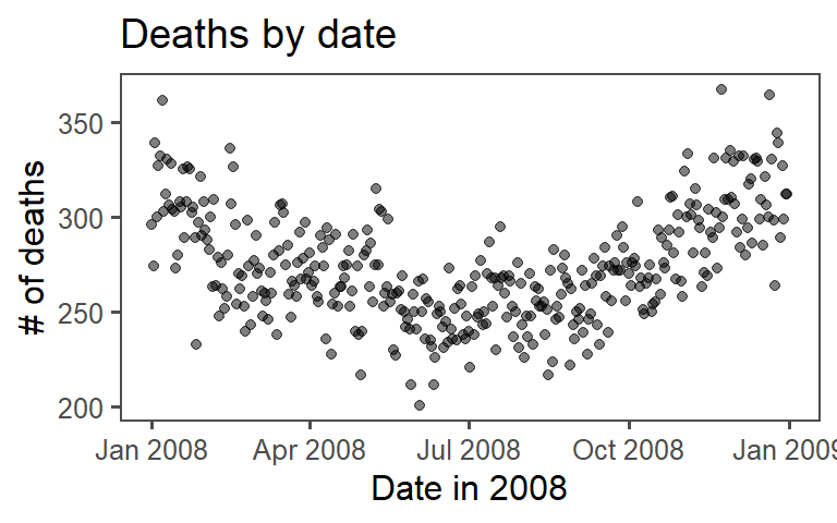 

6.7.3 More extensive data wrangling

• Read the Ebola data directly from GitHub into your R session. Call the dataframe ebola.
• Use dplyr functions to create a tidy dataset. First, change it from “wide” data to “long” data. Name the new column with the key variable and the new column with the values count. The first few lines of the “long” version of the dataset should look like this:

## # A tibble: 6 × 4
##   Date       Day variable           count
##   <chr>    <dbl> <chr>              <dbl>
## 1 1/5/2015   289 Cases_Guinea        2776
## 2 1/5/2015   289 Cases_Liberia         NA
## 3 1/5/2015   289 Cases_SierraLeone  10030
## 4 1/5/2015   289 Cases_Nigeria         NA
## 5 1/5/2015   289 Cases_Senegal         NA
## 6 1/5/2015   289 Cases_UnitedStates    NA

• Convert the Date column to a Date class.
• Use the separate function to separate the variable column into two columns, type (“Cases” or “Deaths”) and country (“Guinea”, “Liberia”, etc.). At this point, the data should look like this:

## # A tibble: 6 × 5
##   Date         Day type  country      count
##   <date>     <dbl> <chr> <chr>        <dbl>
## 1 2015-01-05   289 Cases Guinea        2776
## 2 2015-01-05   289 Cases Liberia         NA
## 3 2015-01-05   289 Cases SierraLeone  10030
## 4 2015-01-05   289 Cases Nigeria         NA
## 5 2015-01-05   289 Cases Senegal         NA
## 6 2015-01-05   289 Cases UnitedStates    NA

• Use the pivot_wider function to convert the data so you have separate columns for the two variables of numbers of Cases and Deaths. At this point, the dataframe should look like this:

## # A tibble: 6 × 5
##   Date         Day country      Cases Deaths
##   <date>     <dbl> <chr>        <dbl>  <dbl>
## 1 2015-01-05   289 Guinea        2776   1786
## 2 2015-01-05   289 Liberia         NA     NA
## 3 2015-01-05   289 SierraLeone  10030   2977
## 4 2015-01-05   289 Nigeria         NA     NA
## 5 2015-01-05   289 Senegal         NA     NA
## 6 2015-01-05   289 UnitedStates    NA     NA

• Remove any observations where counts of both cases and deaths are missing for that country on that date.
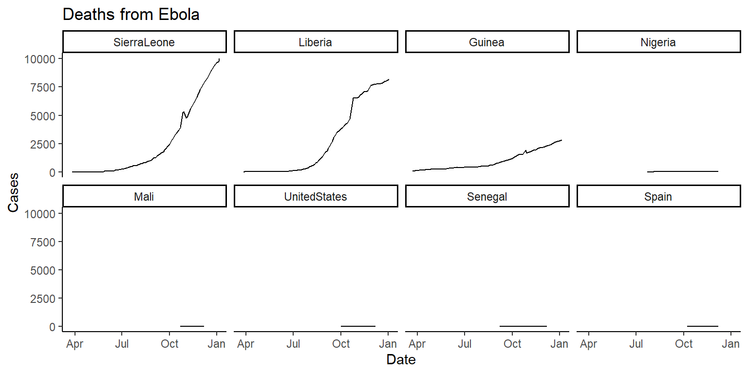
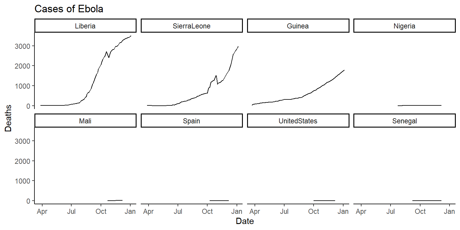
• Now that your data is tidy, create one plot showing Ebola cases by date, faceted by country, and one showing Ebola deaths by date, also faceted by country. Try using the option scales = "free_y" in the facet_wrap function and see how that changes these graphs. Discuss with your group the advantages and disadvantages of using this option when creating these small multiple plots. The plots should look something like this (if you’re using the scales = "free_y" option):

• Based on these plots, what would your next questions be about this data before you used it for an analysis?
• Can you put all of the steps of this cleaning process into just a few “chained” code pipelines using %>%?
• If you have extra time (super-challenge!): There is a function called fct_reorder in the forcats package that can be used to reorder the levels of a factor in a dataframe based on another column in the same dataframe. This function can be very useful for using a meaningful order when plotting. We’ll cover the forcats package in a later class, but today check out the help file for fct_reorder and see if you can figure out how to use it to reorder the small multiple plots in order of the maximum number of cases or deaths (for the two plots respectively) in each country. You’ll be able to do this by changing the code in facet_wrap from ~ country to ~ fct_reorder(country, ...), but with the ... replaced with certain arguments. If you’re getting stuck, try running the examples in the fct_reorder helpfile to get a feel for how this function can be used when plotting. The plots will look something like this:

6.7.3.1 Example R code

Read the data in using read_csv.

ebola_url <- paste0("https://github.com/geanders/RProgrammingForResearch/",
              "raw/master/data/country_timeseries.csv")
ebola <- read_csv(ebola_url)

head(ebola)

## # A tibble: 6 × 18
##   Date         Day Cases_Guinea Cases_Liberia Cases_SierraLeone Cases_Nigeria
##   <chr>      <dbl>        <dbl>         <dbl>             <dbl>         <dbl>
## 1 1/5/2015     289         2776            NA             10030            NA
## 2 1/4/2015     288         2775            NA              9780            NA
## 3 1/3/2015     287         2769          8166              9722            NA
## 4 1/2/2015     286           NA          8157                NA            NA
## 5 12/31/2014   284         2730          8115              9633            NA
## 6 12/28/2014   281         2706          8018              9446            NA
## # ℹ 12 more variables: Cases_Senegal <dbl>, Cases_UnitedStates <dbl>,
## #   Cases_Spain <dbl>, Cases_Mali <dbl>, Deaths_Guinea <dbl>,
## #   Deaths_Liberia <dbl>, Deaths_SierraLeone <dbl>, Deaths_Nigeria <dbl>,
## #   Deaths_Senegal <dbl>, Deaths_UnitedStates <dbl>, Deaths_Spain <dbl>,
## #   Deaths_Mali <dbl>

Change the data to long data using the pivoter_longer function from tidyr:

ebola <- ebola %>%
  pivot_longer(cols = c(-Date, -Day), names_to = "variable", values_to = "count")
head(ebola)

## # A tibble: 6 × 4
##   Date       Day variable           count
##   <chr>    <dbl> <chr>              <dbl>
## 1 1/5/2015   289 Cases_Guinea        2776
## 2 1/5/2015   289 Cases_Liberia         NA
## 3 1/5/2015   289 Cases_SierraLeone  10030
## 4 1/5/2015   289 Cases_Nigeria         NA
## 5 1/5/2015   289 Cases_Senegal         NA
## 6 1/5/2015   289 Cases_UnitedStates    NA

Convert Date to a date class:

ebola <- ebola %>%
         mutate(Date = mdy(Date))
head(ebola)

## # A tibble: 6 × 4
##   Date         Day variable           count
##   <date>     <dbl> <chr>              <dbl>
## 1 2015-01-05   289 Cases_Guinea        2776
## 2 2015-01-05   289 Cases_Liberia         NA
## 3 2015-01-05   289 Cases_SierraLeone  10030
## 4 2015-01-05   289 Cases_Nigeria         NA
## 5 2015-01-05   289 Cases_Senegal         NA
## 6 2015-01-05   289 Cases_UnitedStates    NA

Split variable into type and country:

ebola <- ebola %>% 
  separate(variable, c("type", "country"), sep = "_")

head(ebola)

## # A tibble: 6 × 5
##   Date         Day type  country      count
##   <date>     <dbl> <chr> <chr>        <dbl>
## 1 2015-01-05   289 Cases Guinea        2776
## 2 2015-01-05   289 Cases Liberia         NA
## 3 2015-01-05   289 Cases SierraLeone  10030
## 4 2015-01-05   289 Cases Nigeria         NA
## 5 2015-01-05   289 Cases Senegal         NA
## 6 2015-01-05   289 Cases UnitedStates    NA

Convert the data so you have separate columns for the two variables of numbers of Cases and Deaths:

ebola <- pivot_wider(ebola, names_from = type, values_from = count)
head(ebola)

## # A tibble: 6 × 5
##   Date         Day country      Cases Deaths
##   <date>     <dbl> <chr>        <dbl>  <dbl>
## 1 2015-01-05   289 Guinea        2776   1786
## 2 2015-01-05   289 Liberia         NA     NA
## 3 2015-01-05   289 SierraLeone  10030   2977
## 4 2015-01-05   289 Nigeria         NA     NA
## 5 2015-01-05   289 Senegal         NA     NA
## 6 2015-01-05   289 UnitedStates    NA     NA

Remove any observations where counts of cases or deaths are missing for that country:

ebola <- filter(ebola, !is.na(Cases) & !is.na(Deaths))
head(ebola)

## # A tibble: 6 × 5
##   Date         Day country     Cases Deaths
##   <date>     <dbl> <chr>       <dbl>  <dbl>
## 1 2015-01-05   289 Guinea       2776   1786
## 2 2015-01-05   289 SierraLeone 10030   2977
## 3 2015-01-04   288 Guinea       2775   1781
## 4 2015-01-04   288 SierraLeone  9780   2943
## 5 2015-01-03   287 Guinea       2769   1767
## 6 2015-01-03   287 Liberia      8166   3496

Now that your data is tidy, create one plot showing ebola cases by date, faceted by country, and one showing ebola deaths by date, also faceted by country:

ggplot(ebola, aes(x = Date, y = Cases)) + 
        geom_line() + 
        facet_wrap(~ country, ncol = 4) + 
        theme_classic()

ggplot(ebola, aes(x = Date, y = Deaths)) + 
        geom_line() + 
        facet_wrap(~ country, ncol = 4) + 
        theme_classic()

Try using the option scales = "free_y" in the facet_wrap() function (in the gridExtra package) and see how that changes these graphs:

ggplot(ebola, aes(x = Date, y = Cases)) + 
        geom_line() + 
        facet_wrap(~ country, ncol = 4, scales = "free_y") + 
        theme_classic()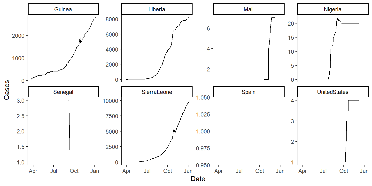

ggplot(ebola, aes(x = Date, y = Deaths)) + 
        geom_line() + 
        facet_wrap(~ country, ncol = 4, scales = "free_y") + 
        theme_classic()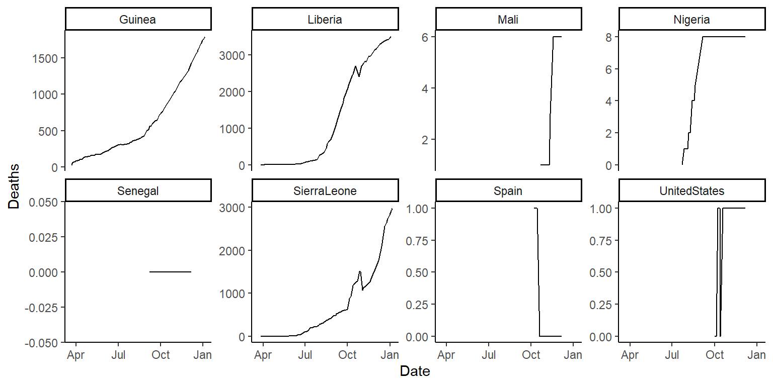

Put all of the steps of this cleaning process into just a few “chaining” calls.

ebola <- read_csv(ebola_url) %>%
         pivot_longer(cols = c(-Date, -Day), names_to = "variable", values_to = "count") %>%
         mutate(Date = mdy(Date)) %>%
         separate(variable, c("type", "country"), sep = "_") %>%
         pivot_wider(names_from = type, values_from = count) %>%
         filter(!is.na(Cases) & !is.na(Deaths))

ggplot(ebola, aes(x = Date, y = Cases)) + 
        geom_line() + 
        facet_wrap(~ country, ncol = 4) + 
        theme_classic()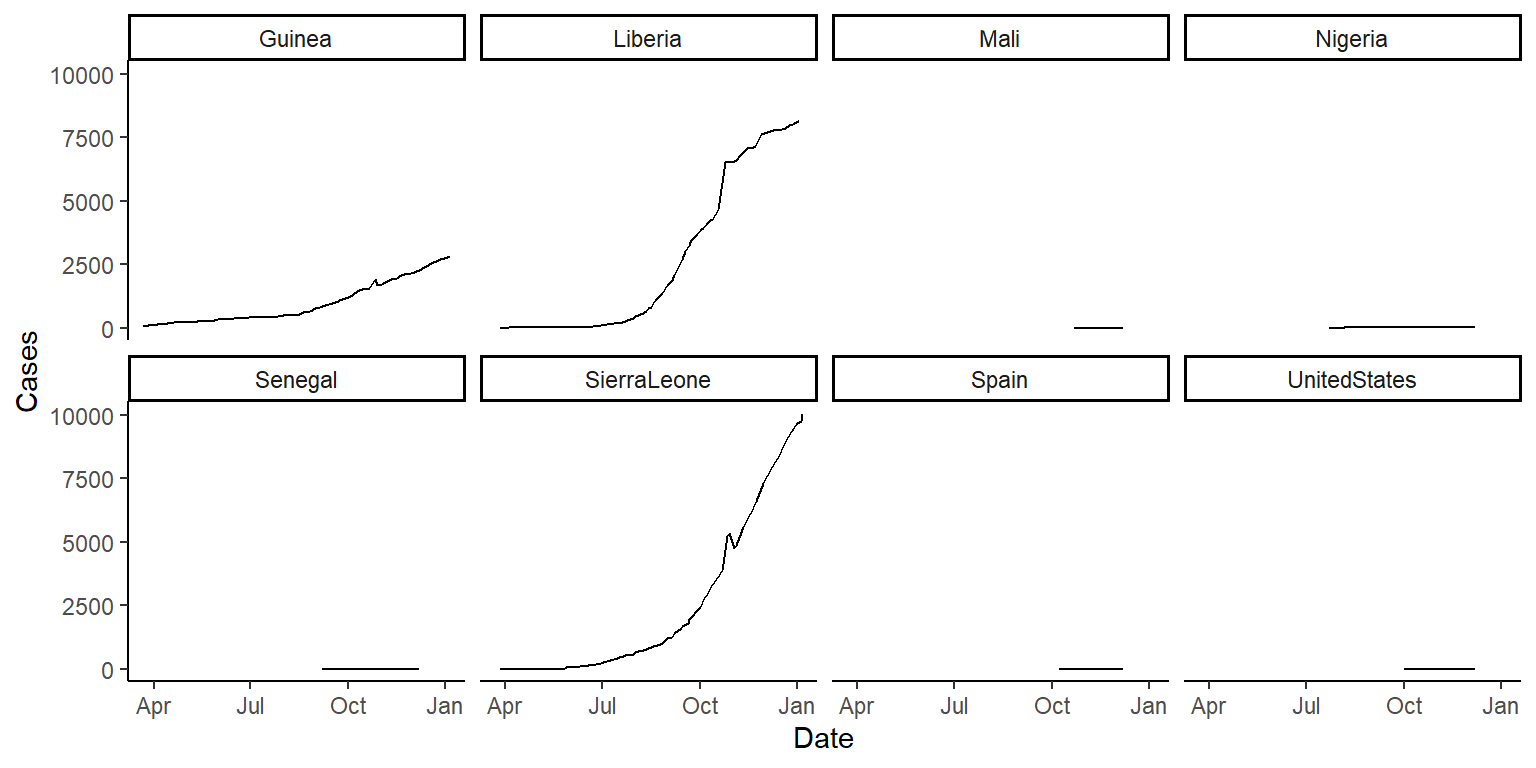

ggplot(ebola, aes(x = Date, y = Deaths)) + 
        geom_line() + 
        facet_wrap(~ country, ncol = 4) + 
        theme_classic()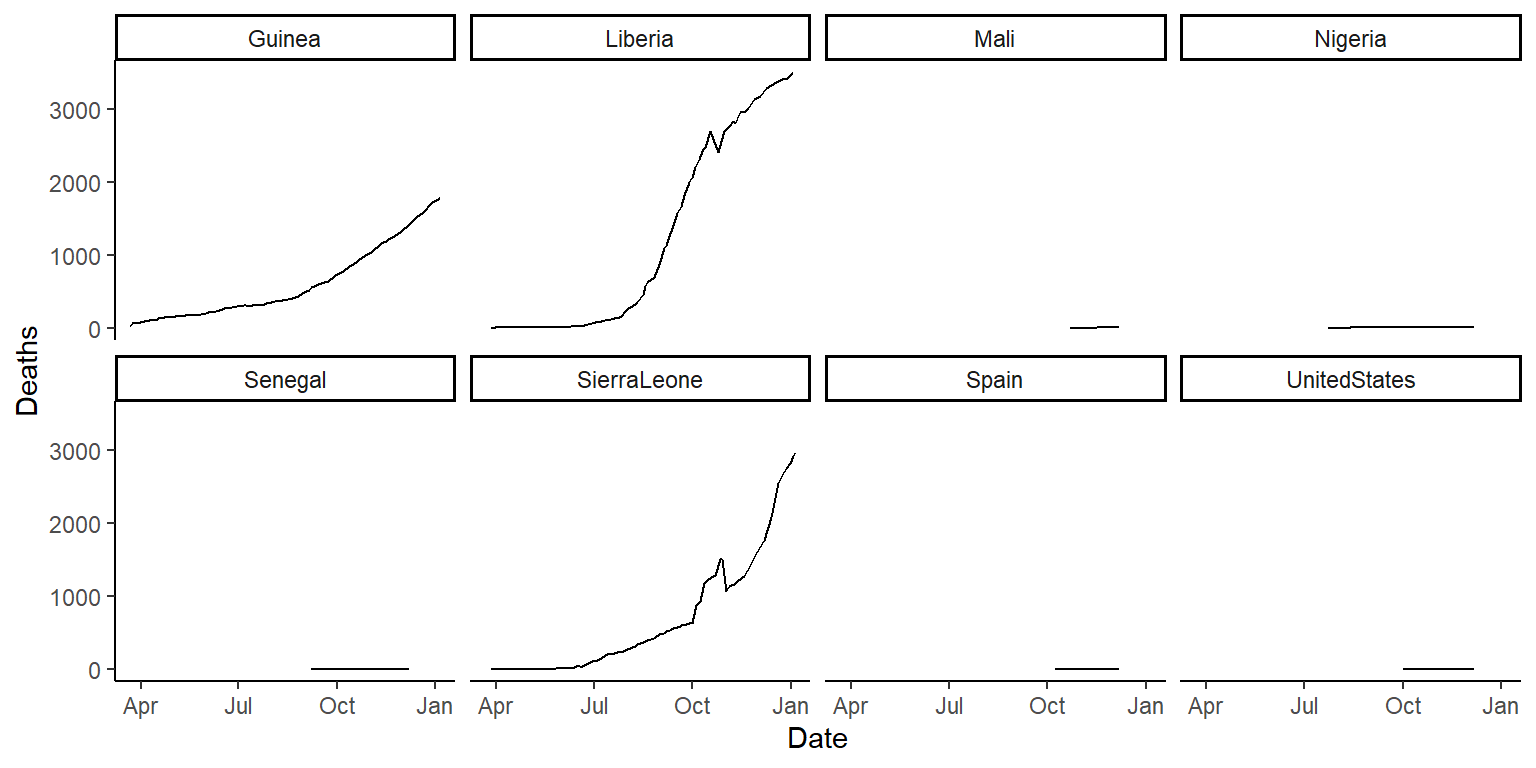

Use the fct_reorder function inside the facet_wrap function call to reorder the small-multiple graphs.

library(forcats)
ggplot(ebola, aes(x = Date, y = Cases)) + 
        geom_line() + 
        facet_wrap(~ fct_reorder(country, Cases, .fun = max, .desc = TRUE),
                   ncol = 4) + 
        theme_classic()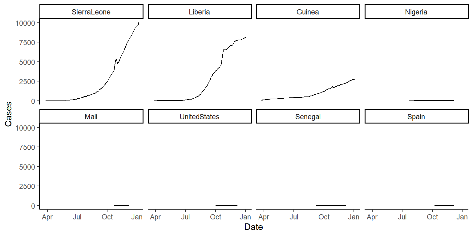

ggplot(ebola, aes(x = Date, y = Deaths)) + 
        geom_line() + 
        facet_wrap(~ fct_reorder(country, Deaths, .fun = max, .desc = TRUE),
                   ncol = 4) + 
        theme_classic()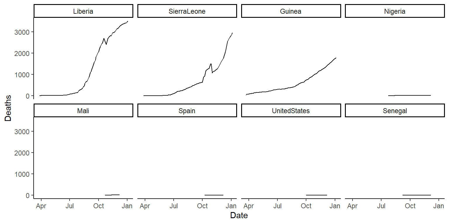

6.7.4 Tidying VADeaths data

R comes with a dataset called VADeaths that gives death rates per 1,000 people in Virginia in 1940 by age, sex, and rural / urban.

• Use data("VADeaths") to load this data. Make sure you understand what each column and row is showing – use the helpfile (?VADeaths) if you need.
• Go through the three characteristics of tidy data and the five common problems in untidy data that we talked about in class. Sketch out (you’re welcome to use the whiteboards) what a tidy version of this data would look like.
• Open a new R script file. Write R code to transform this dataset into a tidy dataset. Try using a pipe chain, with %>% and tidyverse functions, to clean the data.
• Use the tidy data to create the following graph:

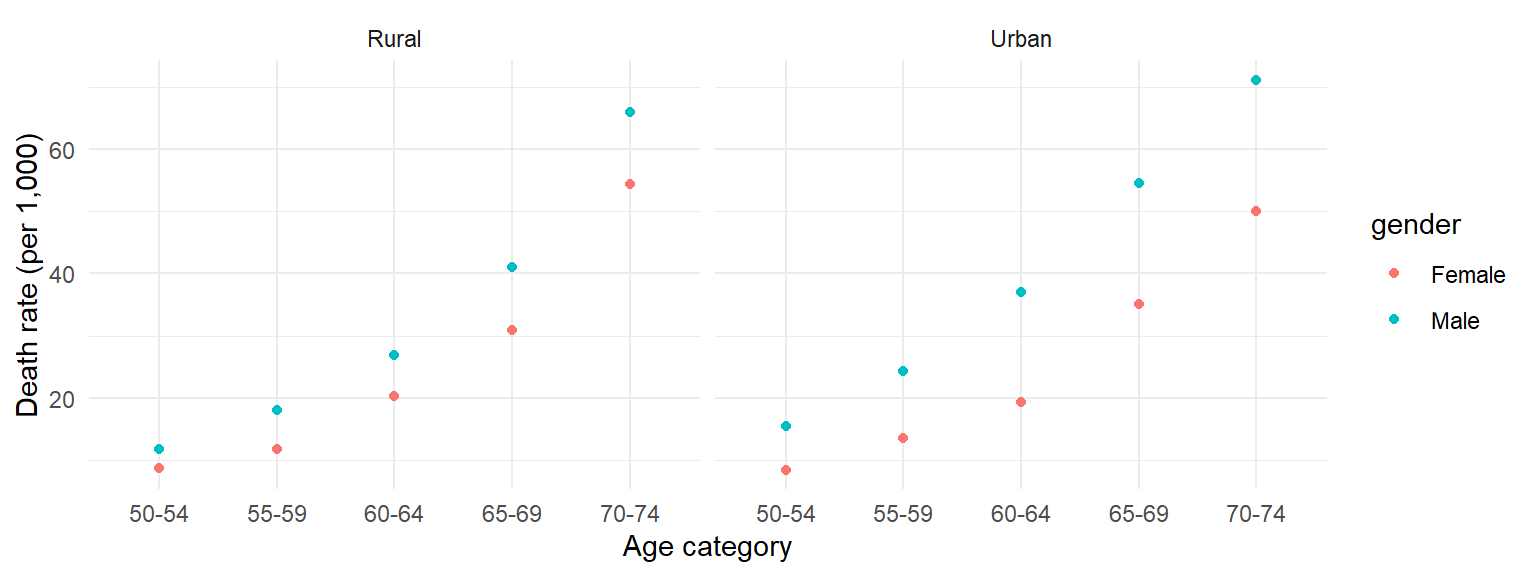
There is no example R code for this – try to figure out the code yourselves. I go over a solution in the following video. You may find the RStudio Data Wrangling cheatsheet helpful for remembering which tidyverse functions do what.

Download a pdf of the lecture slides for this video.

6.7.5 Baby names

In the Fall 2018 session, we seem to have an unusually high percent of the class with names that start with an “A” or “K”. In this part of the exercise, we’ll see if we can figure out whether the proportion of “A” and “K” names is unusual.

There is a package on CRAN called babynames with data on baby names by year in the United States, based on data from the U.S.’s Social Security Administration. We will use this data to compare the proportion of “A” and “K” names in our class with the proportion in these baby names. We’ll also do a few other things to explore this data.

• First, check out patterns in your own name. Is your name included in this dataset? Has your name been used for males and females? How have the patterns in the proportion of babies with your name, for both males and females, changed over time (use a plot to look at this)?
• In the year you were born, what were the 5 most popular baby names for males and females? Try to come up with some attractive ways (figures and tables) to show this.

6.7.5.1 Example R code

Install and load the babynames package and its “babynames” dataframe:

# install.packages("babynames")
library(babynames)
data("babynames")

Remember that you can use ?babynames to find out more about this dataframe.

Check out patterns in your own name. Is your name included in this dataset? You can use filter to create a subset of this data where you’ve filtered down to just the rows with your name. To see if your name ever shows up, you can use count on this dataframe—if your name never shows up, then you will have 0 rows in the new dataframe. As long as there’s at least one row, your name shows up somewhere. (If your name is not in here, try your middle or last name, or the name of a fictional character you like, for the rest of these exercises.)

my_name <- babynames %>% 
  filter(name == "Brooke")
my_name %>% 
  count()

## # A tibble: 1 × 1
##       n
##   <int>
## 1   174

Has your name been used for males and females? To figure this out, you can group the dataset with rows with your name by the sex column and then use count to count the number of rows in the dataset for males and females. If your name has only been used for one gender, then only one row will result from running this code (for an example, try my first name, “Georgiana”).

my_name %>% 
  group_by(sex) %>% 
  count()

## # A tibble: 2 × 2
## # Groups:   sex [2]
##   sex       n
##   <chr> <int>
## 1 F        82
## 2 M        92

How have the patterns in the proportion of babies with your name, for both males and females, changed over time (use a plot to look at this)? To check this out, I recommend you create a plot of the proportion of babies with your name (prop) versus year (year). You can use color to show these patterns for males and females separately. I’ve done some extra things here to (1) relabel the sex factor, so the label shows up with clearer names and (2) change the labels for the x-, y-, and color scales.

library(forcats)
my_name %>% 
  mutate(sex = fct_recode(sex, Male = "M", Female = "F")) %>% 
  ggplot(aes(x = year, y = prop, color = sex)) + 
  geom_line() + 
  labs(x = "Year", y = "Proportion of babies\nof each sex named 'Brooke'",
       color = "")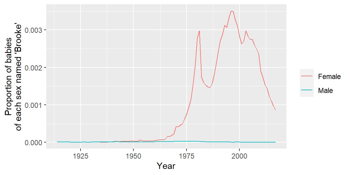

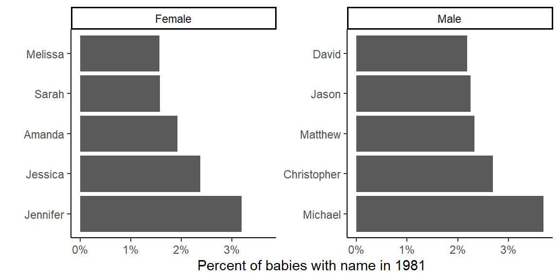
In the year you were born, what were the 5 most popular baby names for males and females?

top_my_year <- babynames %>% 
  filter(year == 1981) %>% 
  group_by(sex) %>% 
  arrange(desc(prop)) %>% 
  slice(1:5)

top_my_year

## # A tibble: 10 × 5
## # Groups:   sex [2]
##     year sex   name            n   prop
##    <dbl> <chr> <chr>       <int>  <dbl>
##  1  1981 F     Jennifer    57049 0.0319
##  2  1981 F     Jessica     42532 0.0238
##  3  1981 F     Amanda      34374 0.0192
##  4  1981 F     Sarah       28173 0.0158
##  5  1981 F     Melissa     28000 0.0157
##  6  1981 M     Michael     68765 0.0369
##  7  1981 M     Christopher 50233 0.0270
##  8  1981 M     Matthew     43330 0.0233
##  9  1981 M     Jason       41932 0.0225
## 10  1981 M     David       40659 0.0218

If you’d like to show this in a prettier way, you could show this as a table:

library(knitr)
top_my_year %>% 
  mutate(rank = 1:n()) %>% # Since the data is grouped by sex, this will rank
                           # separately for females and males
  ungroup() %>% # You have to ungroup before you can run `mutate` on `sex`
  mutate(sex = fct_recode(sex, Male = "M", Female = "F"),
         percent = round(100 * prop, 1),
         percent = paste(percent, "%", sep = "")) %>% 
  select(sex, rank, name, percent) %>% 
  kable()

sex	rank	name	percent
Female	1	Jennifer	3.2%
Female	2	Jessica	2.4%
Female	3	Amanda	1.9%
Female	4	Sarah	1.6%
Female	5	Melissa	1.6%
Male	1	Michael	3.7%
Male	2	Christopher	2.7%
Male	3	Matthew	2.3%
Male	4	Jason	2.3%
Male	5	David	2.2%

You could also show it as a figure:

library(scales)
top_my_year %>% 
  ungroup() %>% 
  mutate(name = fct_reorder(name, prop, .desc = TRUE),
         sex = fct_recode(sex, Male = "M", Female = "F")) %>% 
  ggplot(aes(x = name)) + 
  geom_bar(aes(weight = prop)) + 
  coord_flip() + 
  labs(x = "", y = "Percent of babies with name in 1981") + 
  theme(legend.position = "top") + 
  scale_y_continuous(labels = percent) + 
  facet_wrap(~ sex, scales = "free_y") + 
  theme_classic()